 Chapter 4 - NovoDeblur plugins
 Contents
- 4.1 The Contrast-limited histogram equalization (CLAHE) plugin
- 4.2 The Unsharp masking plugin
- 4.3 The Destriper plugin
- 4.4 The Color channel combiner plugin
The NovoDeblur GUI includes several plugins for image post-processing, such as Contrast-Limited Histogram Equalization (CLAHE), unsharp masking, and stripe artifact removal. These tools help fine-tune the appearance of deconvolved image stacks and can also be used as alternative processing options for stacks that are not suitable for deconvolution. The Color channel combiner plugin allows users to merge image stacks recorded with different color filters into a single RGB stack using either additive or subtractive color mixing.
The contrast-limited histogram equalization (CLAHE) plugin
Contrast-Limited Adaptive Histogram Equalization (CLAHE) is an image-processing technique widely used in biomedical imaging to enhance contrast. Unlike standard histogram equalization, which applies one global adjustment to the full image, CLAHE operates on small regions called tiles and adjusts contrast locally. By applying a contrast limit ("clip limit") to each local histogram, CLAHE reduces noise amplification. The result is improved local contrast, especially in areas with varying brightness, while minimizing over-enhancement in more uniform regions. The CLAHE plugin in NovoDeblur guides users through this process step by step.
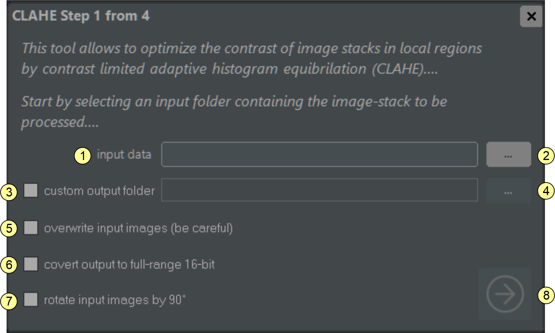
Figure 4.1 CLAHE tool. The interface guides you through the contrast-enhancement process in four steps. In step 1, specify the input folder and basic settings. (1) input folder path display. (2) input folder selector. (3) custom output folder checkbox. (4) output folder selector. (5) overwrite source images checkbox. (6) if checked, output images are scaled to the full 16-bit range (brightest pixel becomes 65535). (7) if checked, images are rotated clockwise by 90° before loading. (8) proceed to next step button.
On the first page (figure 4.1), specify the source stack location (1-2) and basic parameters (3-7). If checkbox (3) is enabled, you can define a custom output folder using button (4). Otherwise, the tool creates an output folder named "CLAHEprocessed" inside the source folder. If checkbox (5) is enabled, source data are overwritten and no output folder is created, so use this option with care. By default, processed images are saved as 16-bit TIFF files spanning the full intensity range (darkest voxel becomes 0, brightest becomes 65535). If checkbox (7) is enabled, input images are rotated clockwise by 90° before loading. Click proceed (8) to continue.
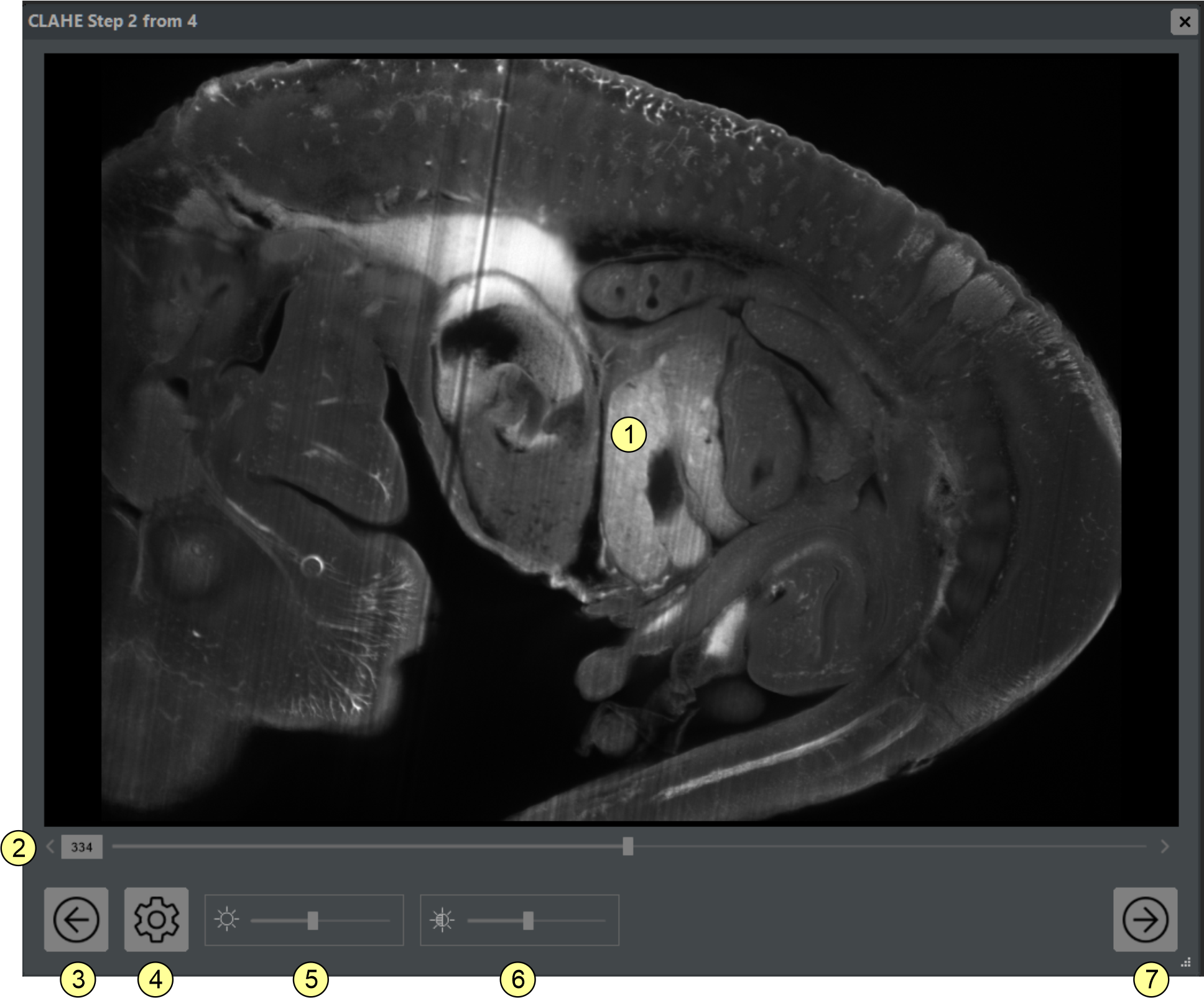
On the second page (figure 4.2), review the current stack. Use the mouse wheel and left mouse button for zooming and panning. Scroll through slices with slider (2). Clicking the settings icon (4) opens the CLAHE parameter window (figure 4.3). You can also adjust display brightness and contrast with sliders (5) and (6). Click proceed (7) to compute a contrast-enhanced preview and continue.
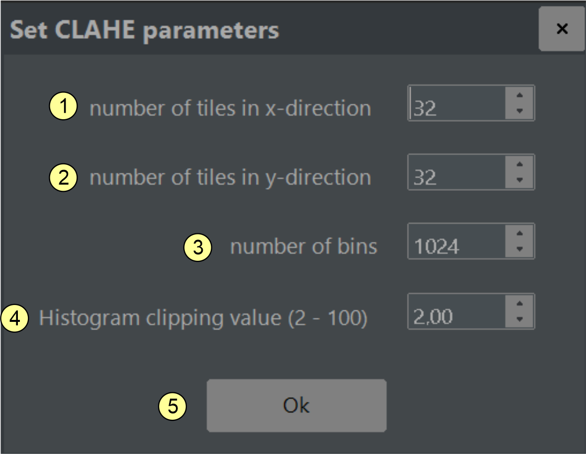
Figure 4.3 CLAHE parameter window. Set the number of tiles in the X and Y directions (1-2), the number of histogram bins (3), and the clipping value that limits contrast amplification (4). Click the close window button (5) to return.
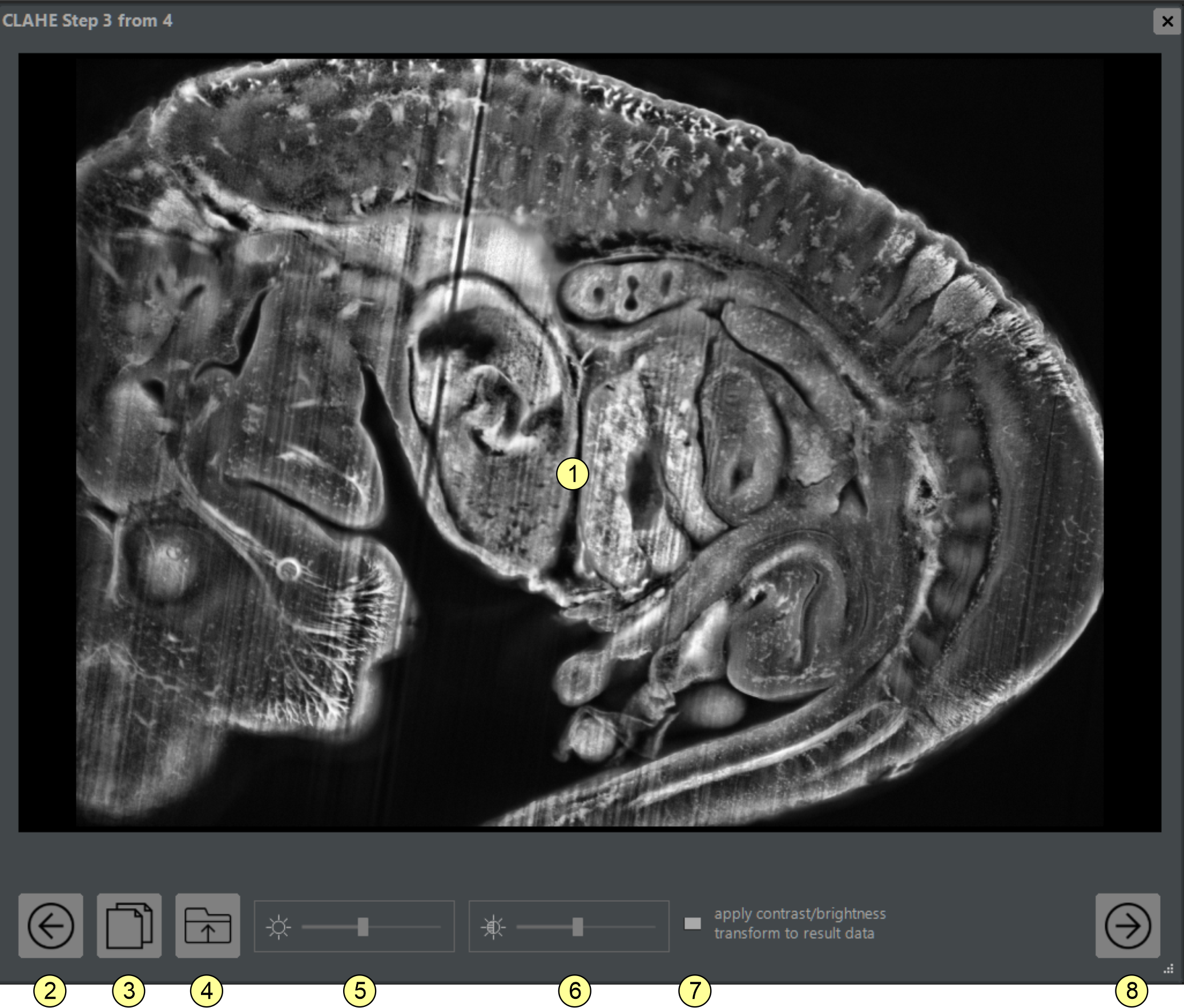
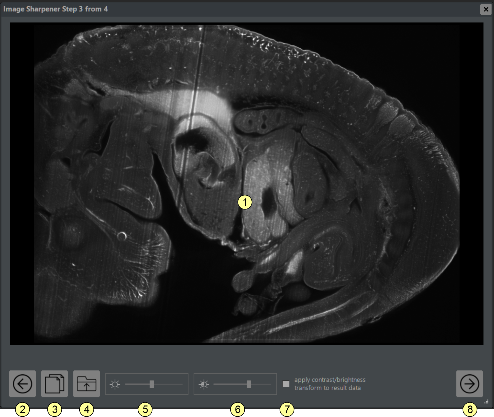
On page three (figure 4.4), review the processed image. Compare it with the corresponding raw image by clicking button (3). Adjust display contrast and brightness with sliders (5) and (6). If checkbox (7) is enabled, these adjustments are also applied to the final output; otherwise, they affect only on-screen visualization. Click button (8) to continue.
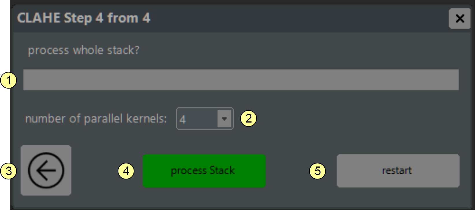
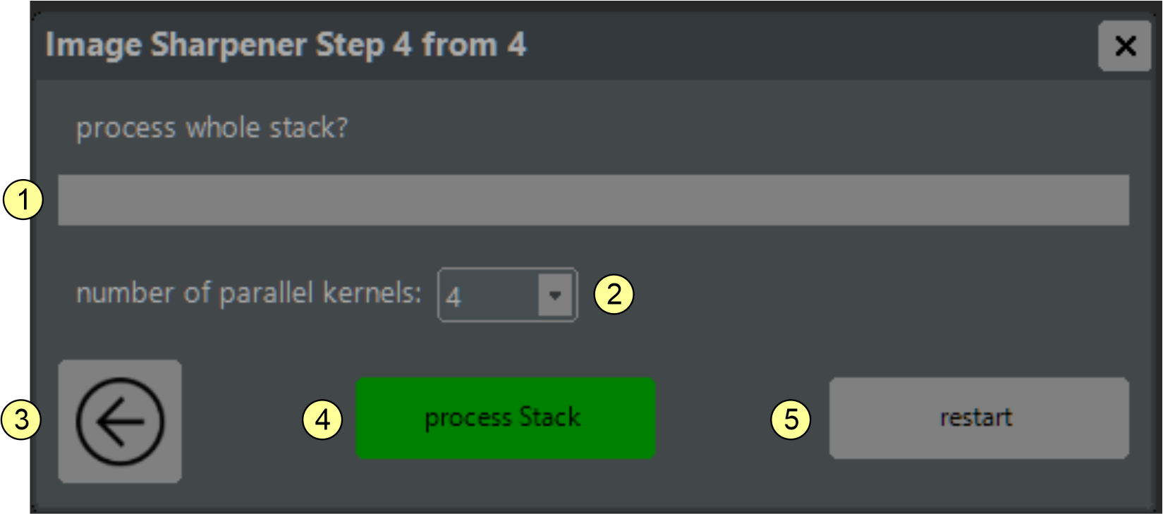
On the final page (figure 4.5), start processing the full source stack. Set the number of parallel worker threads with combo box (2). This value cannot exceed the number of available CPU cores and is capped at 12. Click button (4) to start processing. You can abort a running task by holding the ESC key. After completion, click button (5) to restart the tool for the next dataset.
The unsharp masking plugin
Unsharp masking is an image-sharpening technique that enhances edge definition and visual clarity. The algorithm creates a blurred ("unsharp") version of the image and subtracts it from the original to boost high-frequency content. The enhanced edge information is then added back, producing a sharper image. Key parameters are amount (overall strength), radius (scale of enhanced edges), and threshold (limits sharpening to significant edges to reduce noise amplification). The NovoDeblur sharpening tool guides users through this process step by step.
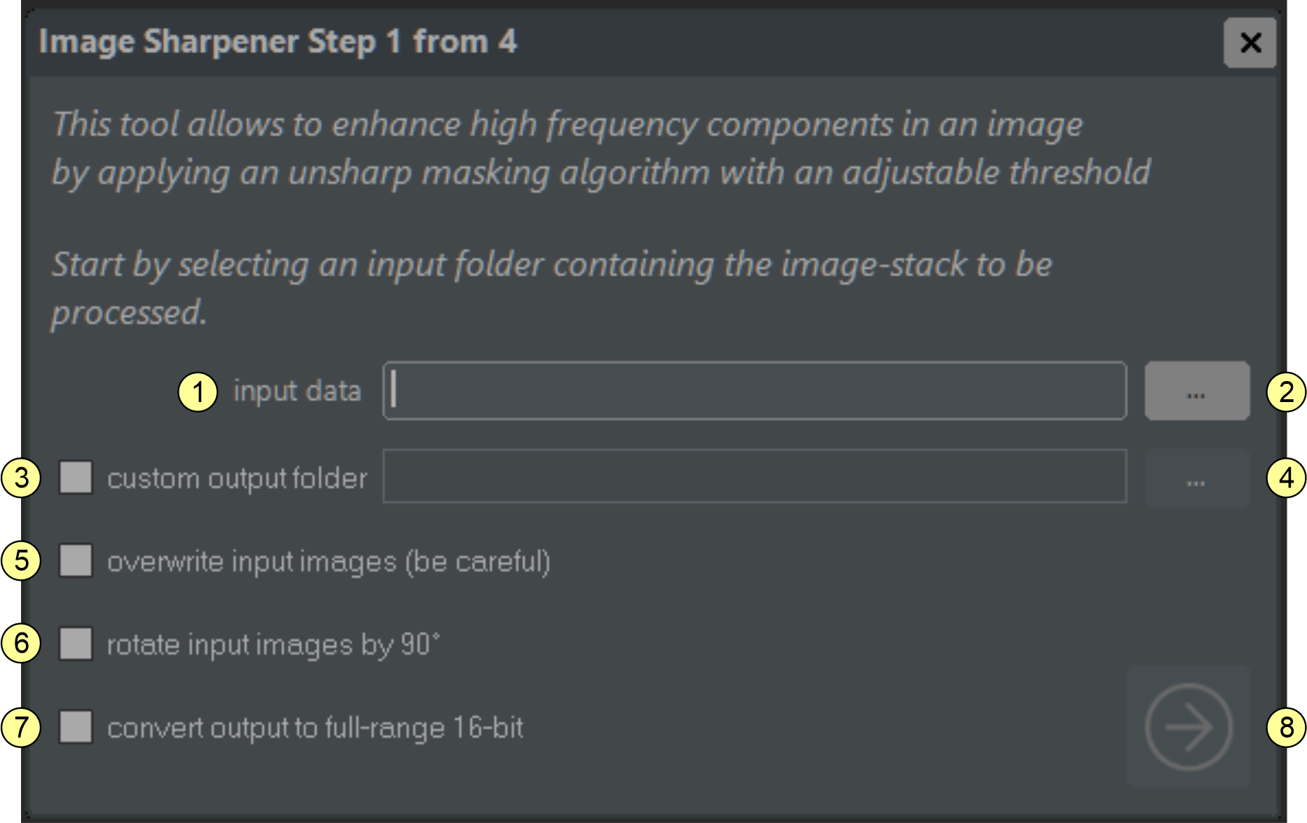
On the first page (figure 4.6), specify the source data location (1-2). If checkbox (3) is enabled, you can define a custom output folder using button (4). Otherwise, the tool creates a folder named "sharpened" inside the source folder. If checkbox (5) is enabled, source data are replaced by processed data. By default, output is stored in the same format as input. If checkbox (6) is enabled, output is saved as full-range 16-bit images. If checkbox (7) is enabled, input images are rotated by 90° before processing. Click proceed (8) to continue.
On the second page (figure 4.7), review the input stack and scroll through slices with slider (2). Open the sharpening parameter dialog (figure 4.8) via button (4). Adjust display contrast and brightness with sliders (5) and (6). Click proceed (7) to compute the sharpened preview and continue.
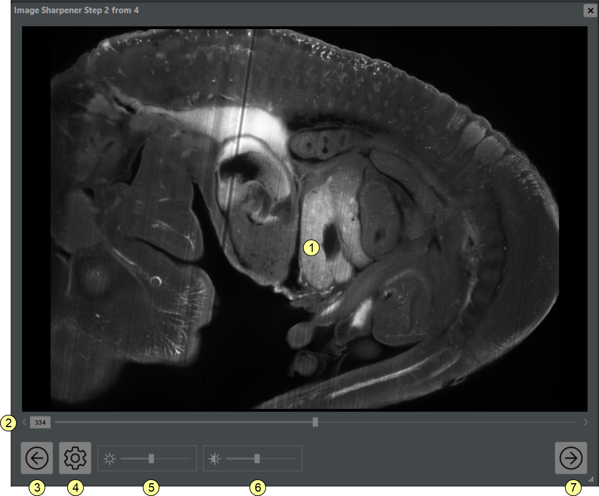
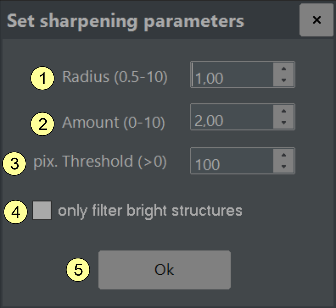
Figure 4.8 Sharpening parameter window. Specify radius (1), amount (2), and threshold (3). If checkbox (4) is checked, only structures located on a darker background are considered for sharpening. Click the close window button (5) to return.
On the third page (figure 4.9), you can review the sharpened image. By clicking button (3), a window opens showing the corresponding raw image for comparison. Adjust contrast and brightness with sliders (5) and (6). If checkbox (7) is checked, changes are applied to the final output images. Otherwise, adjustments only affect the screen representation. Click button (8) to proceed.
On the final page (figure 4.10), start processing the full source stack. Set the number of parallel worker threads with combo box (2). This value is limited to available CPU cores and cannot exceed 12. Click button (4) to start processing. Click button (5) to restart the tool for the next dataset.
The destriper plugin
Dark, unidirectional stripe patterns are a common artifact in light-sheet microscopy, often caused by pigmented structures that partially block the light sheet. The NovoDeblur destriping plugin reduces these artifacts using directional frequency filtering with a pie-slice-shaped mask. This mask selectively attenuates spatial-frequency components in the stripe direction with smooth (tapered) edges. The destriping wizard guides users through the full workflow step by step.
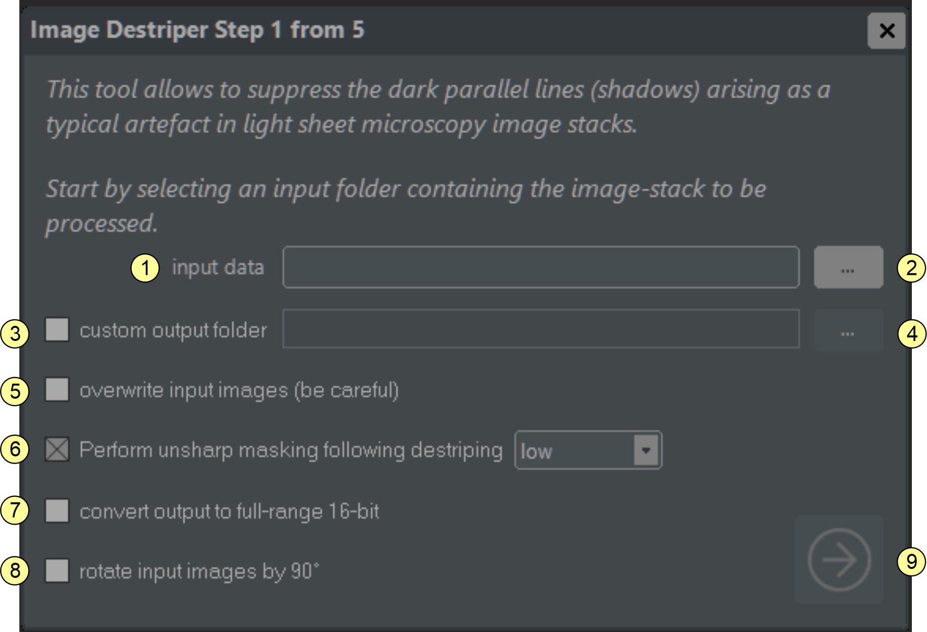
On the start page (figure 4.11), specify the source data location (1-2) and basic parameters (3-8). If checkbox (3) is enabled, you can define a custom output folder; otherwise, a folder named "destriped" is created inside the source folder. If checkbox (5) is enabled, source data are replaced by processed data and no output folder is created, so use this option carefully. If checkbox (6) is enabled, additional unsharp masking is applied after filtering to compensate for blur; strength can be set from low to high. By default, output is saved in the same format as input. If checkbox (7) is enabled, output is converted to full-range 16-bit format. If checkbox (8) is enabled, input images are rotated by 90° after loading. Click proceed (9) to continue.
On the second page (figure 4.12), review the input images and measure stripe direction. Adjust the stripe angle using the sliders at the left (1) and right (2) edges, scroll through images with slider (3), and adjust display brightness/contrast with sliders (5) and (6). The measured angle is shown in (7). Click proceed (8) to continue.
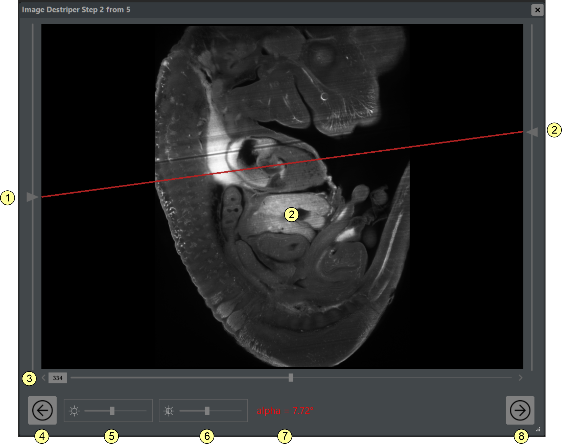
Figure 4.12 Stripe artifact removal tool (step 2 of 5). Determine the stripe angle by aligning the red line parallel to the stripes using the sliders at the left (1) and right (2) edges. (3) Input image stack scroll slider. (4) Return to the previous step button. (5) Brightness slider. (6) Contrast slider. (7) Displayed angle output field. (8) Proceed to next step button.
In step 3, the image power spectrum is shown as a grayscale map (3) with an overlay of the pie-slice filter mask (figure 4.13). Adjust mask rotation with buttons (9-10) and mask shape with sliders (5-8). Tune the filter so that it covers the prominent stripe-related lines in the spectrum (figure 4.14 A1, B1, C1). Guidance for parameters α, w1, w2, d1, and d2 is provided in table 4.1. Press button (11) to process and continue.
| Parameter | Meaning | Optimal Adjustment |
|---|---|---|
| α | Defines stripe direction | Filter mask covers apparent lines in the spectrum |
| w1 | Low frequency direction tolerance | Set as high as necessary |
| w2 | High frequency direction tolerance | Set as high as necessary |
| d1 | Low frequency cutoff | Set as low as necessary |
| d2 | High frequency cutoff | Set as high as necessary |
Table 4.1 Hints for adjusting destriping parameters α, w1, w2, d1, and d2. For severe stripe artifacts, partial reduction (for example 50-75%) is often preferable to avoid introducing secondary artifacts.
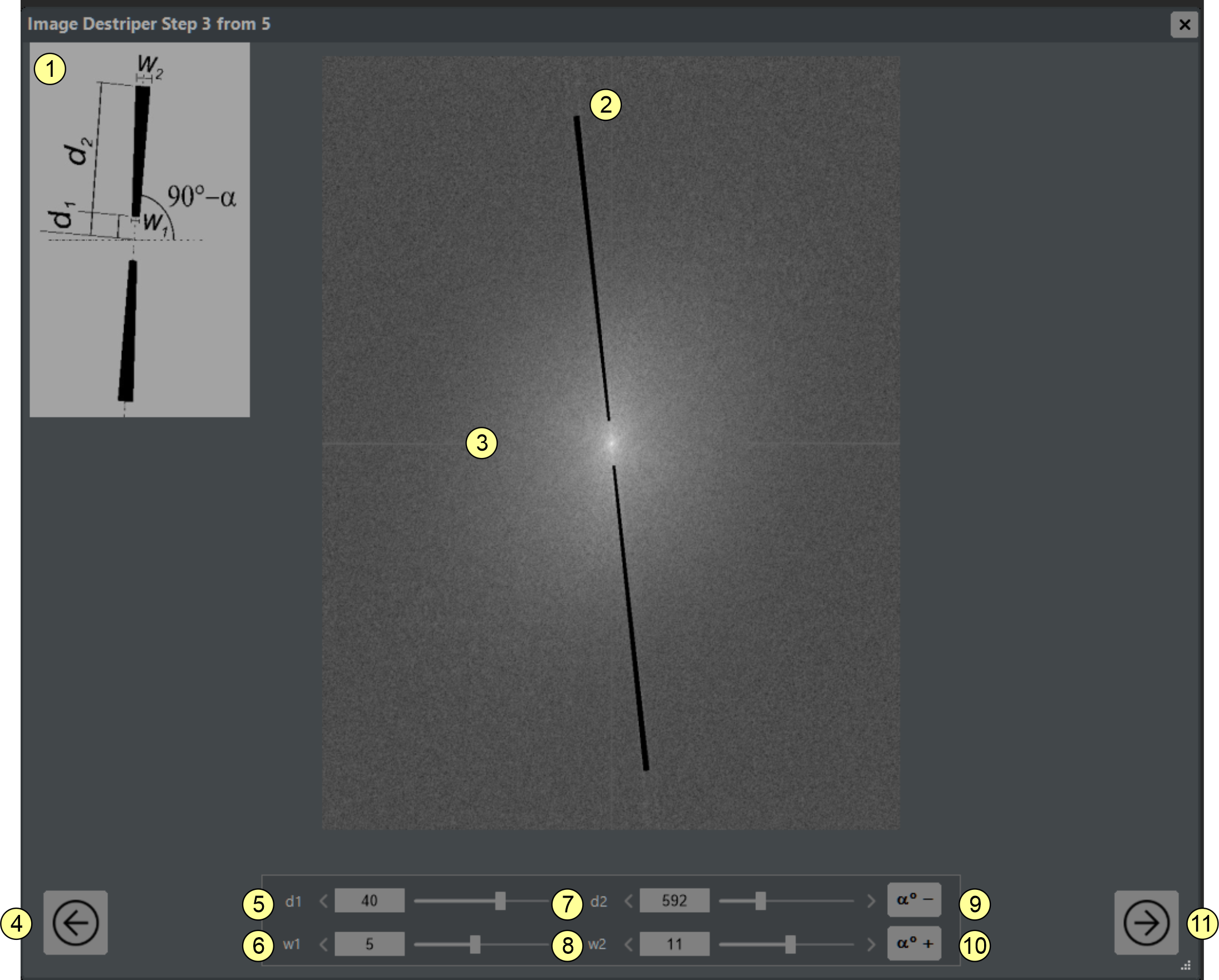
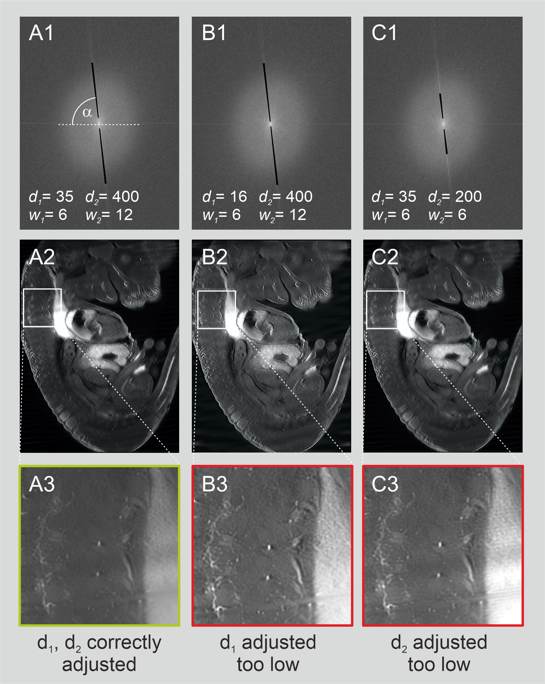
Figure 4.14 Examples of correct parameter adjustment. (A) Stripe artifacts removed. (B) d1 set too low, causing ringing artifacts. (C) d2 set too low, leaving fine stripes.
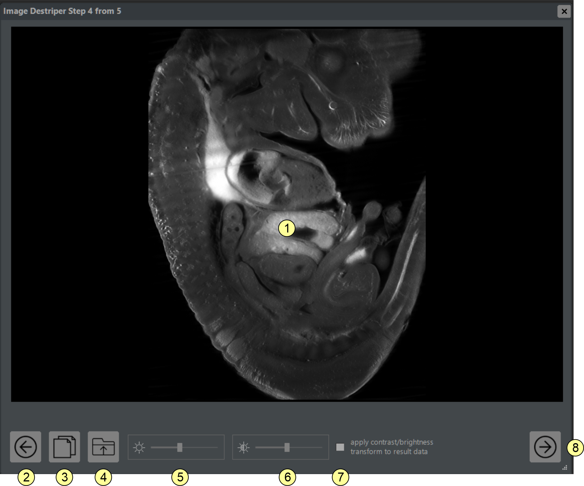
On the fourth page (figure 4.15), review the destriped images. Compare with raw data using button (3). Adjust display contrast and brightness with sliders (5) and (6). If checkbox (7) is enabled, these changes are applied to final output; otherwise, they affect only display. Click button (8) to continue.
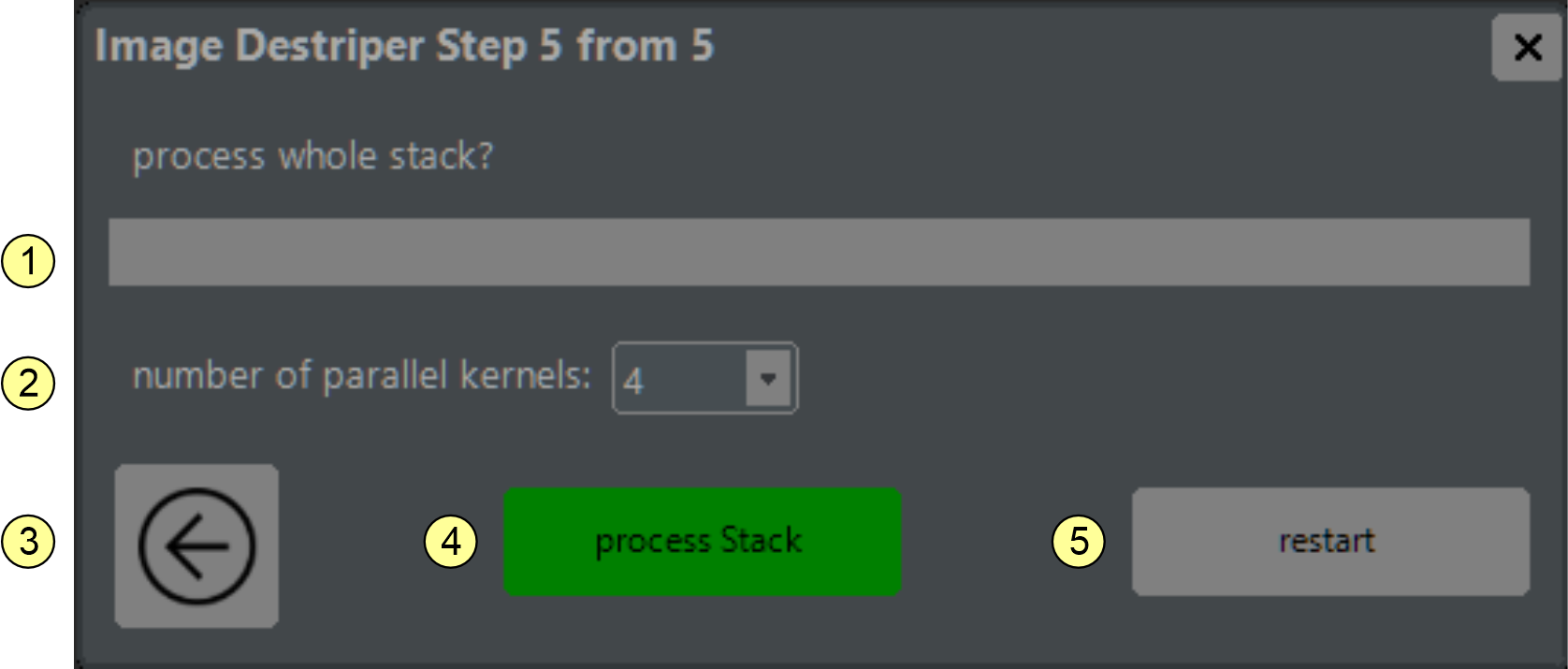
On the final page (figure 4.16), start processing the full source stack. Set the number of computation workers with combo box (2). Click button (4) to start processing. Click button (5) to restart for a new dataset.
The Color channel combiner plugin
The Color channel combiner tool merges up to three stacks of monochromatic TIFF images, each recorded with different chromatic filters, into a single stack of RGB images. Colors can be matched to the peak emission wavelength of a fluorescent dye or selected using a color selector wheel. The mixing mode can be set to additive to simulate light mixing of fluorescent dyes or subtractive for color mixing of absorptive pigments.
Color channel combiner step 1 of 3: Open the Color Channel Combiner from the Plugins menu (figure 4.17). The window contains three display panes (1-3) for previewing one slice from up to three stacks, each assigned to one color channel. Use the Z slider (13) to select the displayed slice. Each input channel must be a 16-bit or 32-bit TIFF stack. All selected folders must contain the same number of images, with filenames ending in equally padded numbers (for example, xx00001.tif, xx00002.tif, ... xx00010.tif). Use buttons (7-9) to select input folders; unassigned channels remain empty.
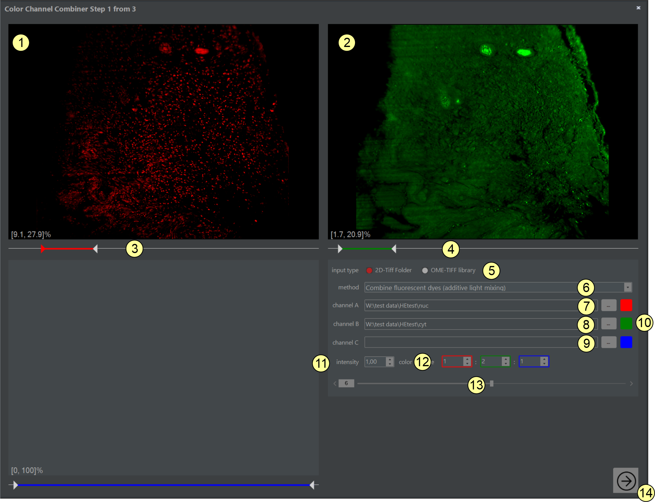
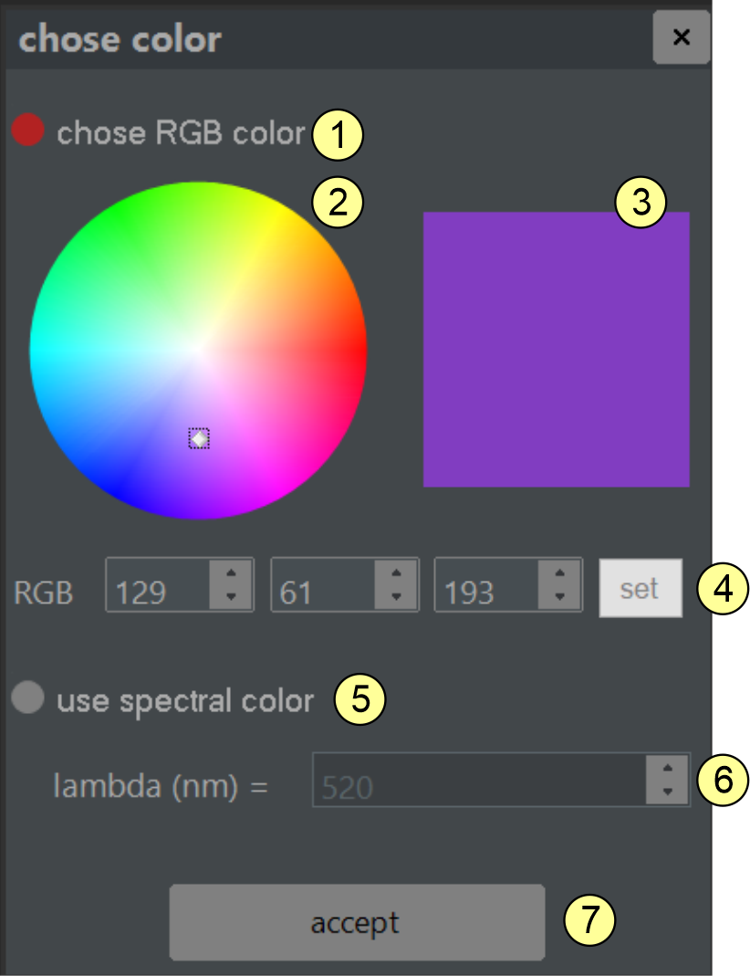
Select colors for each channel by clicking the color buttons (10) and using the color selector window (figure 4.18). Colors can be chosen using the color wheel, specified from a known laser emission line, or set from known RGB values.
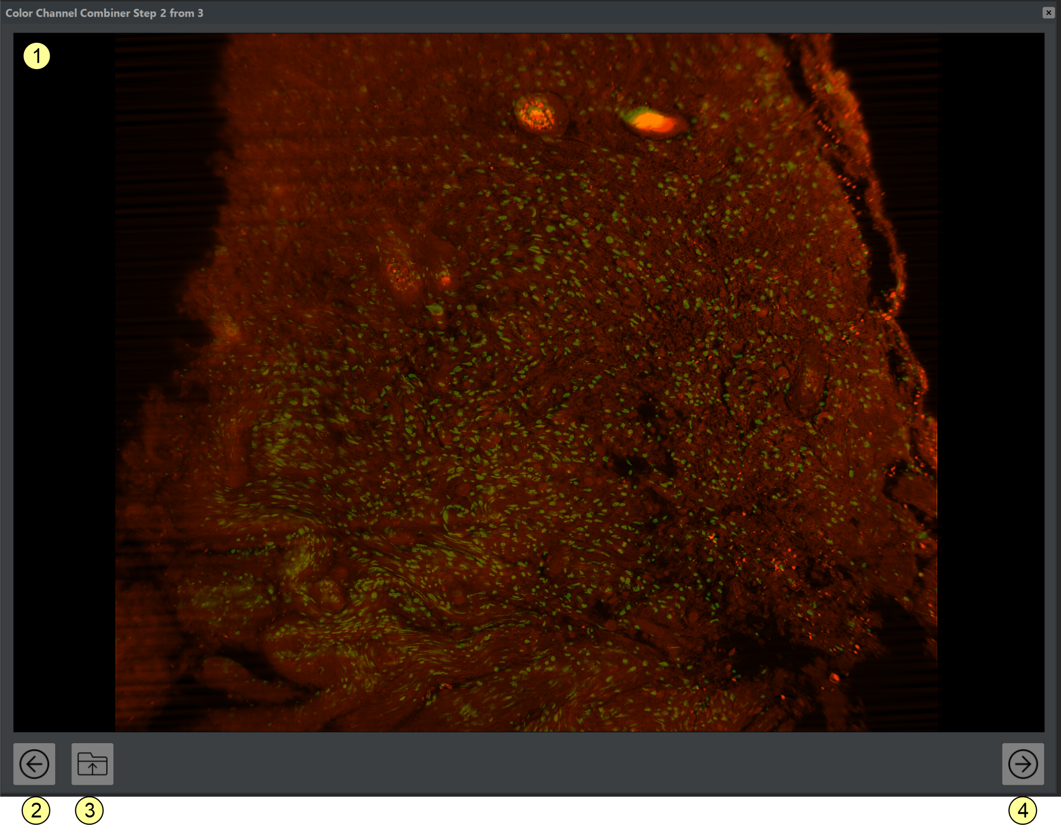
On the second page, the combined RGB image is shown (figure 4.19). You can zoom and pan with the mouse. Click button (2) to return to the previous step, button (3) to save the current image as a 32-bit RGB TIFF, and button (4) to proceed to the final step.
On the final page (figure 4.20), choose the target folder for processed images with button (2); the selected path is shown in (1). Set the number of computation workers with combo box (4). Press button (6) to process the full input stacks. Use button (5) to return to the previous step and button (7) to restart the tool.
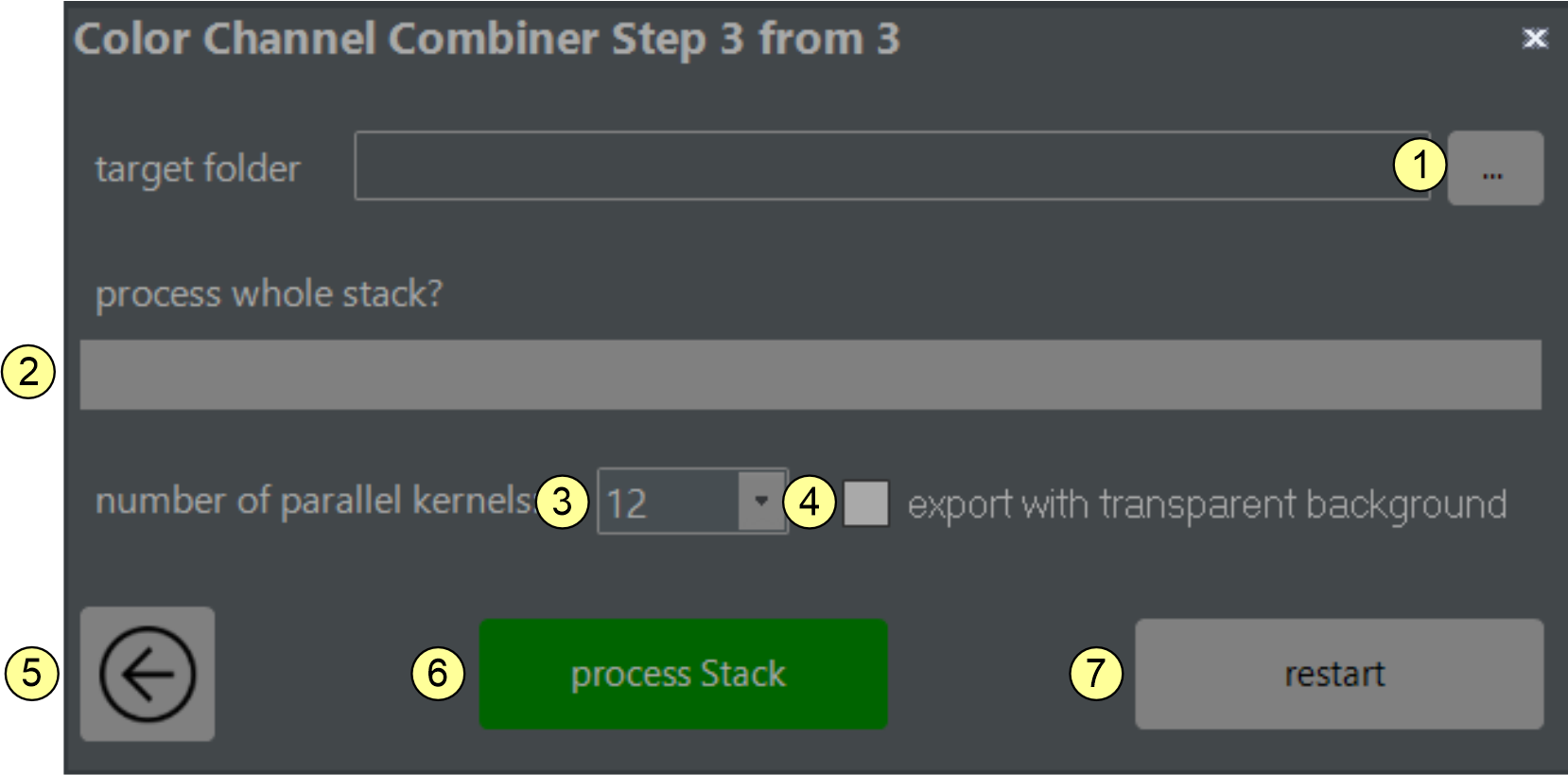
Figure 4.20 Color combiner (step 3 of 3). Specify the target folder and start processing. (1) Select target path here. (2) Progress bar. (3) Maximal number of computation kernels selector. (4) Check if you want to export the combined images with a transparent background. (5) Button to return to the previous step. (6) Start processing button. (7) Restart color channel combiner tool.