 Chapter 5 - Performing an example deconvolution Chapter 5 - Performing an example deconvolution
 5.1 Downloading and uncompressing the demo data set
5.2 Example deconvolution using NovoDeblur GUI
5.3 Example deconvolution using the command line interface
A test data set containing 668 optical slices acquired from an immunostained E12.5 mouse embryo via light sheet microscopy can be downloaded as a ZIP-compressed folder from this link. Before usage, the downloaded ZIP file must be uncompressed into an empty folder on your system, e.g., using the default uncompressing utility provided with Windows. After decompression, the folder should contain 668 sequentially numbered 16-bit TIFF images, each with a resolution of 1392 x 1040 pixels. This data set is also referenced in figure 6.1. The deconvolution of the data set can be performed using either the command-line version or the graphical user interface (NovoDeblurGUI).
The Graphical User Interface (NovoDeblurGUI) allows users to construct command lines required for deconvolution programs, such as lsdeconv.exe for light sheet microscopy stacks, cfdeconv.exe for confocal microscopy stacks, and psfdeconv.exe for deconvolving with a measured point spread function (PSF). Using the GUI, multiple deconvolution jobs can be queued for batch processing, e.g., overnight. Additionally, NovoDeblurGUI includes options for image post-processing (CLAHE, unsharp masking) and stripe artifact removal in light sheet microscopy recordings.
This section details how to deconvolve the demo mouse embryo using NovoDeblurGUI. For more details, refer to Chapter 2.
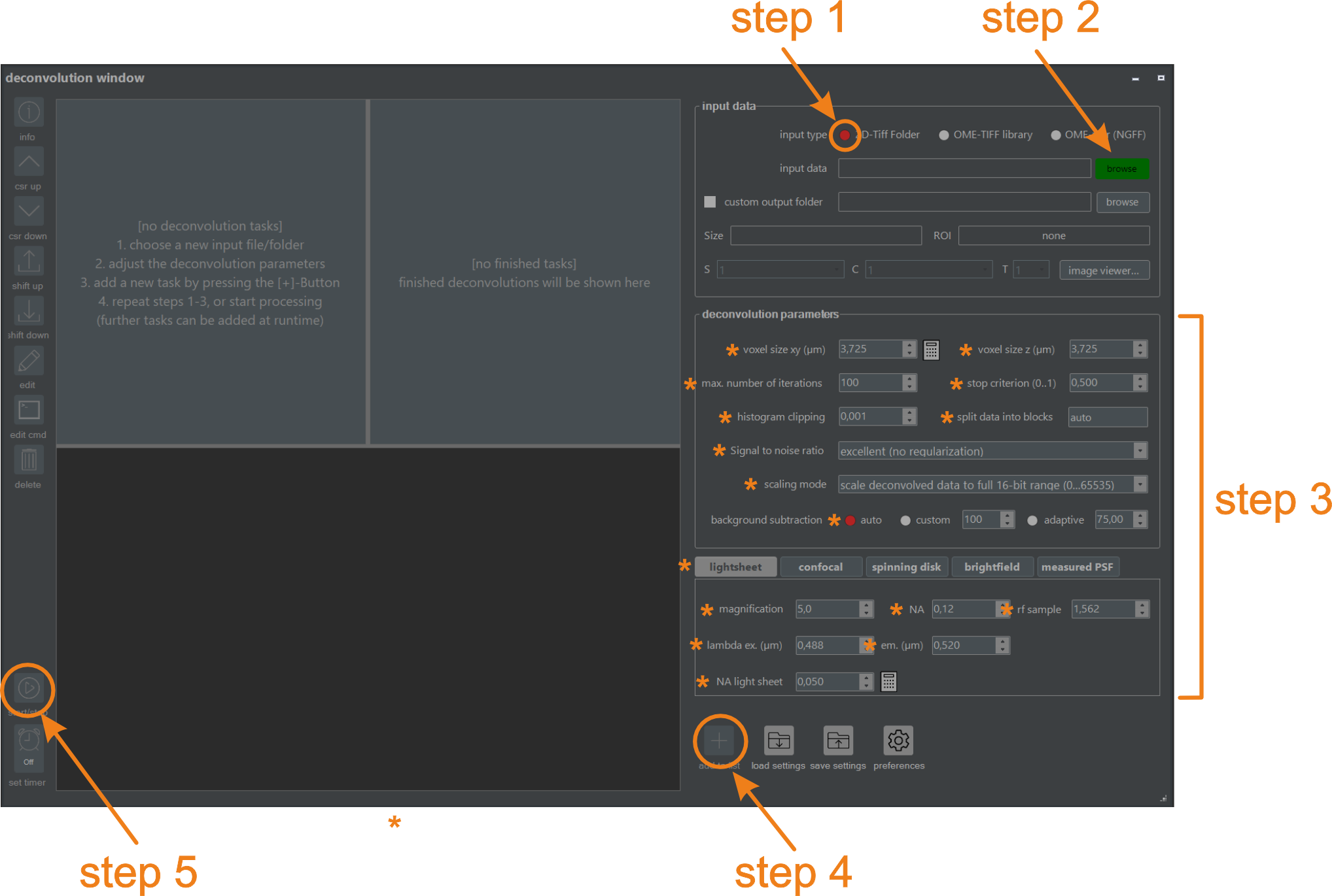
Figure 5.1. Deconvolving the demo embryo using the graphical user interface (NovoDeblurGUI). Perform steps 1-5 sequentially to define and run a new deconvolution. Details for each step are provided below.
NovoDeblur can process image data in either a library format readable using bioformats (e.g., Zeiss, Leica, Olympus) or as a numbered series of TIFF images in a single folder. Since our demo data set is stored in the latter format, select the option "from TIFF-folder" (figure 5.1, Step 1).
If "from library" is selected, a standard file selector box opens after clicking the button indicated in figure 5.1 (Step 2). Otherwise, a folder selection box opens for specifying the directory containing the TIFF images. After selecting the input file or folder, the image inspector opens automatically if activated in the Preferences Menu. If the image inspector opens, it can be closed immediately by clicking the proceed button (figure 5.2), or used to specify a region of interest. For more options provided by the image inspector, refer to Chapter 2.4.3.
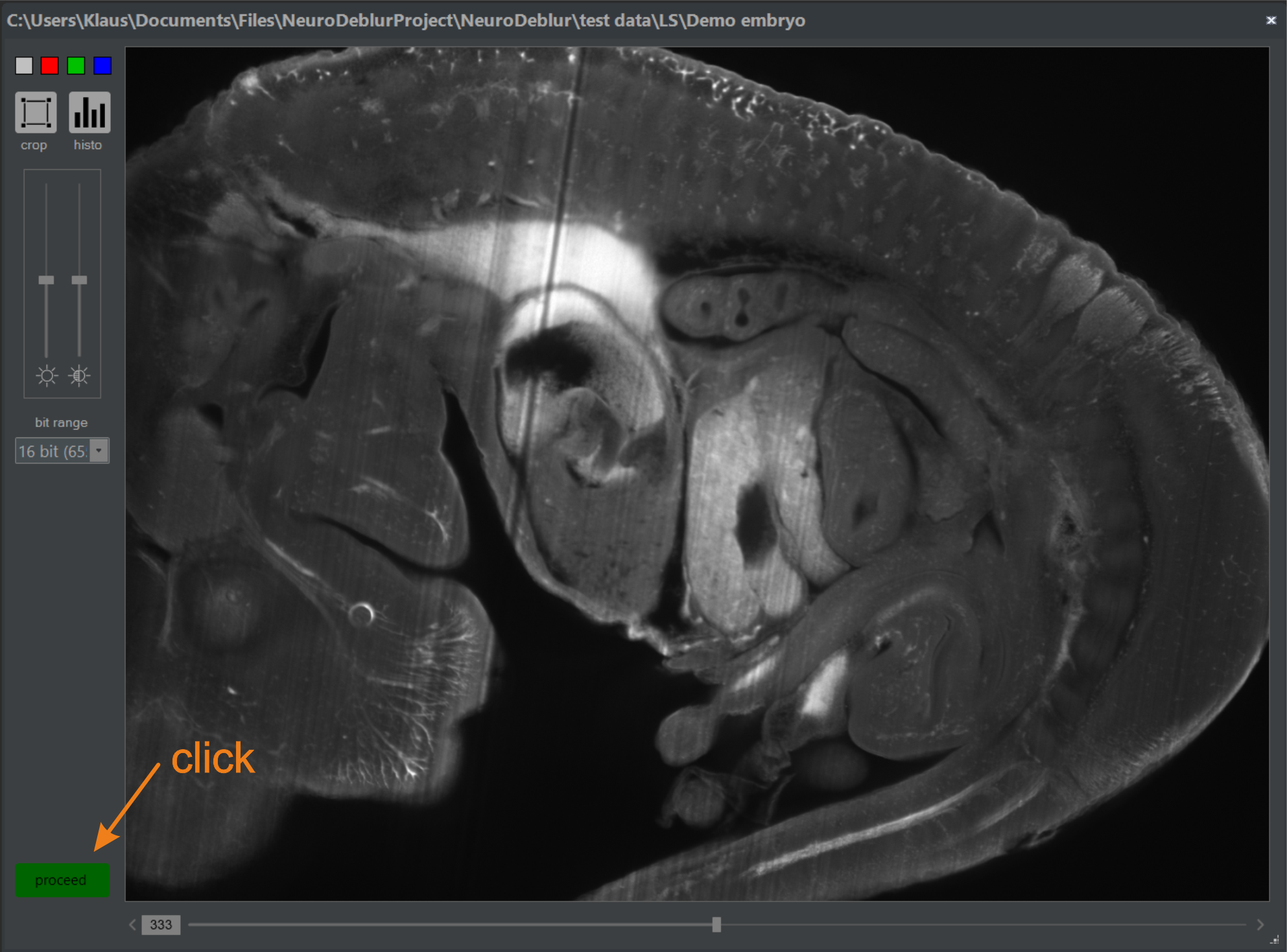
Figure 5.2 image inspector. Select a region of interest (ROI) or a distinct series or image channel from a multi-dimensional image library. Otherwise, close it by clicking the Proceed button.
Specify the deconvolution parameters, such as the numerical aperture (NA) of the objective, the refractive index of the embedding medium, and the voxel size. Select the tab labeled "use light sheet" and enter the parameter values exactly as indicated in figure 5.1 (Step 3). Press the TAB key to move to the next input field after entering each value.
Check if all parameters are specified exactly as depicted in figure 5.1 and press the (+) button (figure 5.1, Step 4) located at the lower right side of the deconvolution window. A new command line is added to the task list window (figure 5.3), and the Start deconvolution button at the lower end of the tool changes its color to green, indicating that the job list can now be processed (figure 5.1, Step 5).
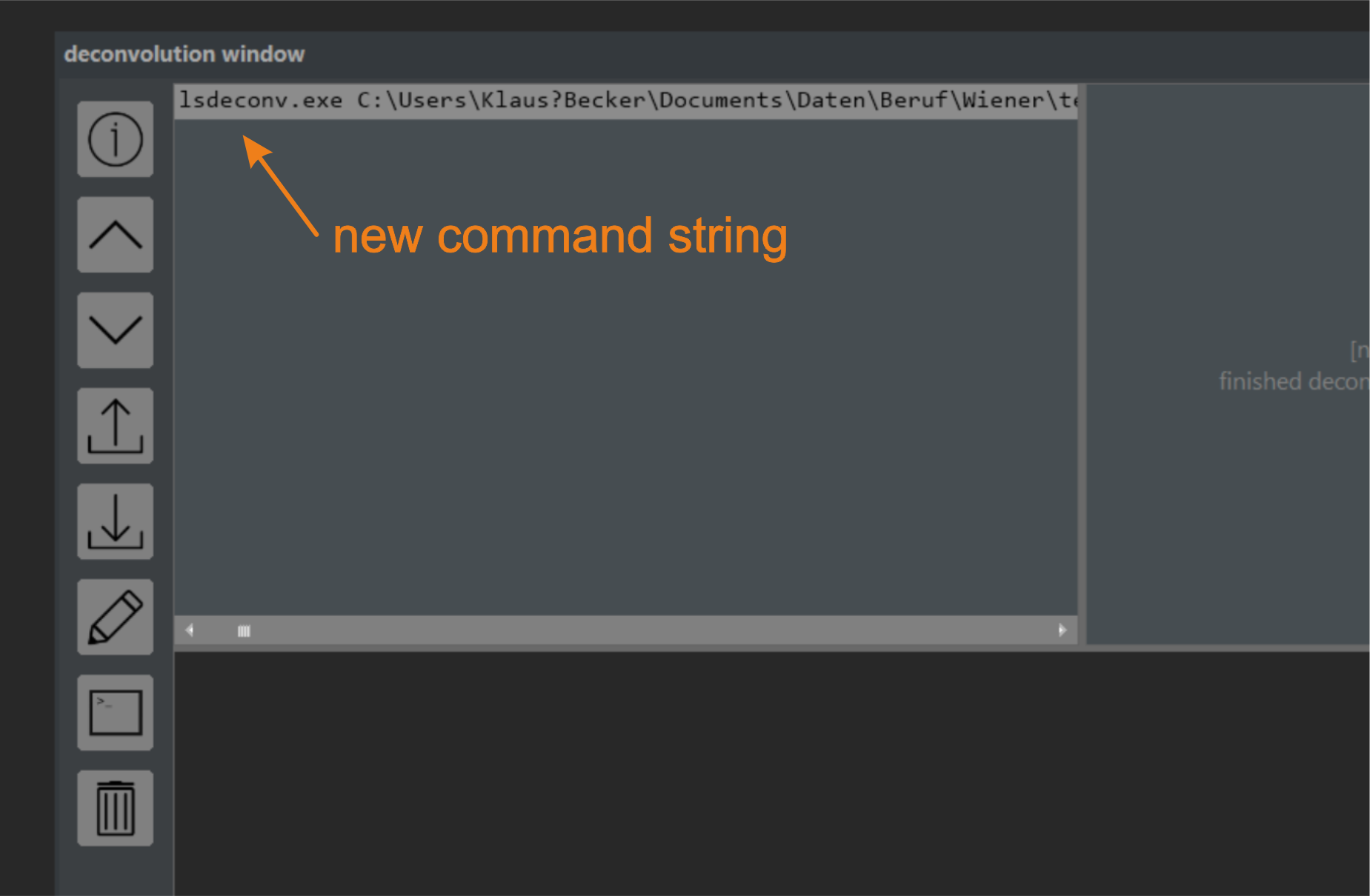
Figure 5.3 The Task Window. Each planned deconvolution creates an entry in the task list window, identical to the command line used in the command line interface.
Press the green Start button at the lower left edge of the deconvolution window to initiate the deconvolution process (figure 5.4). The button turns red once the deconvolution begins. Pressing it again cancels the current task. The processing time varies depending on your hardware and can range from a few minutes on a workstation with a high-end NVIDIA graphics card to a few hours on a basic office computer without GPU acceleration. After deconvolution, the Start button turns gray again, and a small preview image appears in the main window's preview area (figure 5.5).
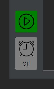
Figure 5.4. The Start Button. Press the green Start button to run the deconvolution. Pressing it again opens a dialog to confirm if you want to cancel the current job list.
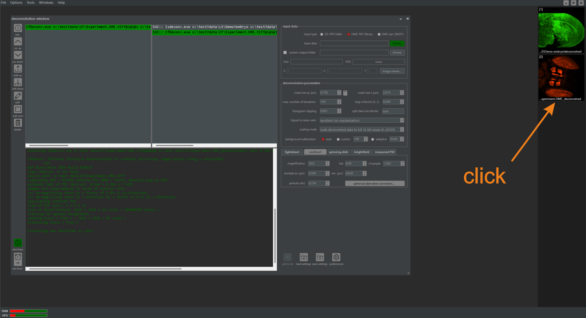
Figure 5.5 Deconvolving the demo embryo using the graphical user interface (NovoDeblurGUI). For each completed deconvolution task, a preview icon is displayed in the preview area. Double-clicking it opens a detailed view of the results.
After the deconvolution is complete, a preview icon is added to the preview area of the main program window (figure 5.5). Double-clicking it opens a result window providing an enlarged view of the deconvolved data set (figure 5.6). Buttons on the left side of the window offer options such as changing the view direction or switching between slice-by-slice and MIP projections from three basic viewing directions. For more details about the result window, refer to Chapter 2.4.4 of this manual. Clicking the encircled button in (figure 5.6) opens a second window showing the raw data for comparison. Zooming or panning in the result window simultaneously alters the content of the raw data window unless this functionality is disabled.
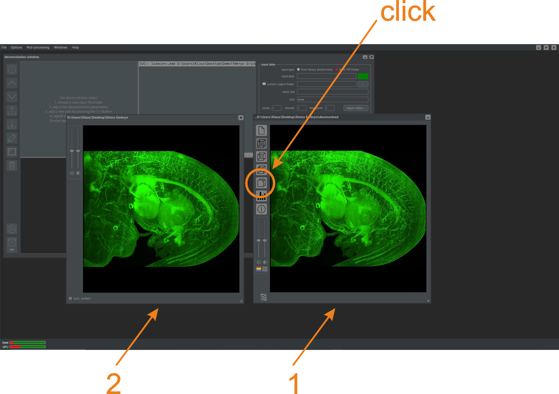
Figure 5.6. Preview (1) and raw data (2) windows. Both windows can be scrolled with the mouse wheel or panned by holding the left mouse button while moving the mouse. Changes in the preview window (1) are synchronously applied to the raw data window (2) unless disabled in the Preferences Window.
This section explains how to perform a deconvolution of the demo mouse embryo using the Deconvolution Console Window.
Step 1: Click the icon labeled NovoDeblur Toolkit in your Start Menu or on your Desktop that was created during the software installation. A new deconvolution window opens, displaying an overview of the available deconvolution and auxiliary commands (figure 5.7).
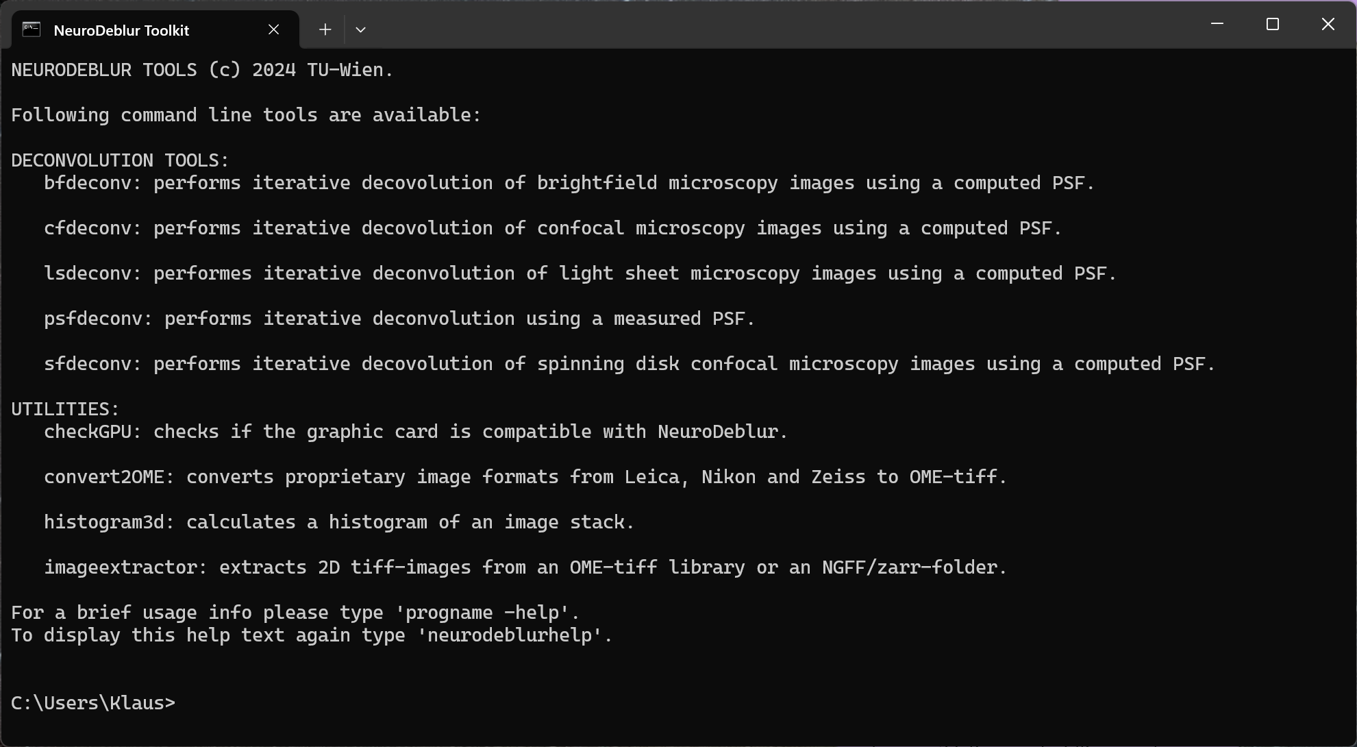
Figure 5.7. The NovoDeblur deconvolution window. The deconvolution window opens after clicking the icon labeled NovoDeblur Deconvolution Toolkit. The window shows an overview of the available commands and utilities.
For a description of all parameters that can be used to invoke a respective deconvolution or utility program, type:
toolname -help or toolname -h where PROGNAME stands for the name of the respective tool (e.g., lsdeconv). Alternatively, refer to Chapter 3 of this documentation.
To display the list of available deconvolution and utility tools again, type:
neurdeblurhelp without any further parameters.
Step 2: Type or copy the following command line into the deconvolution window and press the Enter key:
lsdeconv sourcefolder * auto 1 1 M:10-NA:0.3 0.488 0.520 1.562 0.05 100 0.5 0 0.01 B:75 1 none 0 0 where sourcefolder is the location of the folder containing the demo TIFF images (e.g., "c:\users\me\desktop\my-testdata"). Enclose the entire file path in quotes if it contains spaces. The deconvolution process progress is printed to the console window (figure 5.8).
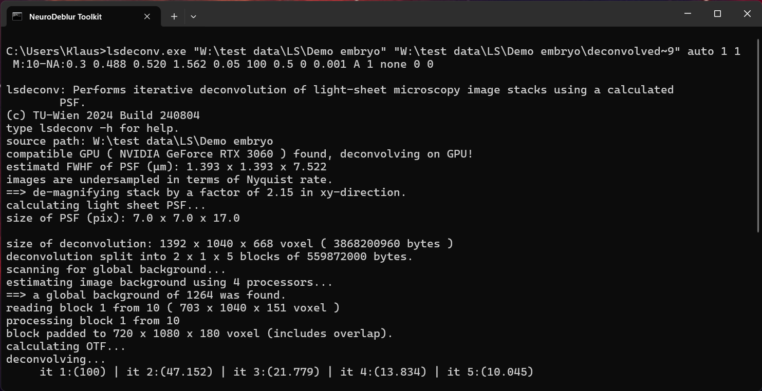
Figure 5.8. Deconvolving the mouse embryo using the deconvolution window. Status messages are printed during the deconvolution process, describing the current step.
The deconvolution process duration depends on your hardware, especially if your system has a compatible graphics card supporting GPU-based deconvolution. For more information about compatible graphics cards, refer to Chapter 1.2. The time required for deconvolving the 668 x 1040 x 1392 voxel stack ranges from 10 minutes (on a high-end computer with a compatible high-end graphics card) to several hours (on a basic office PC without GPU support).
The parameter 'B:75' in the command line ensures adaptive background subtraction using the 'rolling ball' algorithm with a radius of 75 microns. This can significantly improve results but is time-consuming on systems with few processor cores. Choose the radius carefully; if too small, relevant image content may be removed. Alternatively, you can try omitting the adaptive background subtraction by replacing 'B:75' with 'A' (automatic background subtraction). In this case, the lowest pixel intensity value in the stack is subtracted from each intensity value.
lsdeconv sourcefolder * auto 1 1 M:10-NA:0.3 0.488 0.520 1.562 0.05 100 0.5 0 0.01 A 1 none 0 0 To restrict the deconvolution to a sub-volume of the stack, replace 'none' with a string specifying the upper left front and lower right back corners of the sub-volume (e.g., 100-550-300-500-950-500).
lsdeconv sourcefolder * auto 1 1 M:10-NA:0.3 0.488 0.520 1.562 0.05 100 0.5 0 0.01 A 1 100-550-300-500-950-500 0 0 This command generates an output stack of 200 images with a resolution of 400 x 400 pixels, representing a sub-volume starting at coordinates [100, 550, 300] and ending at [500, 950, 500].