Chapter 2 - Working with the graphical user interface
Index Previous Next
2.1 Scheduling deconvolutions
2.2 How to run deconvolution jobs
2.3 Visualizing and inspecting your deconvolution results
2.4 Description of the main NovoDeblur GUI components
2.4.1 The NovoDeblur GUI window
2.4.2 The deconvolution window
2.4.3 The image inspector
2.4.4 The result windows
2.4.5 The preferences dialog window
2.1 Scheduling deconvolutions
Step 1: Specifying new input data
- NovoDeblur can process two types of input data:
- Numbered series of single 8-bit, 16-bit, or 32-bit grayscale tiff-images stored in a common folder.
- Single-file image libraries in the OME-tiff format maintained by the Open Microscopy Environment (OME) Community.
- Additionally, the novel OME-NGFF format is supported, although metadata handling is still under development.
- Common formats such as .cvi from Zeiss and .lif from Leica can be converted using the free FormatsConverter bundled with the software.
The input data type (tiff, OME-tiff, or OME-NGFF) is selected using the input type selector radio buttons at the top of the deconvolution window (figure 2.4, items B-1 and B-2).
- After selecting the input data type, click the file selector button (figure 2.4, item B-4). This opens a dialog box to specify the location of your image data. After confirming the location, the data are checked for readability (only for single tiff-images and unless disabled in the preferences window). If the test passes, the background color of the (+) button (figure 2.4, item B-39) turns green, indicating that the new input data can be added to the deconvolution task list after all parameters have been set up correctly (figure 2.4, item A-9).
- Once a new data location is specified, the image inspector window opens automatically if configured in the preferences window. Otherwise, the image inspector button (figure 2.4, item B-13) can be clicked to manually open the image inspector, e.g., for selecting color channels in multidimensional OME-tiff libraries or restricting the deconvolution to a region of interest (ROI).
Step 2: Defining the deconvolution parameters
- After specifying the input source, choose one of the tabs labeled light sheet, confocal, spinning disk, brightfield, and measured PSF (figure 2.4, items B23 - B25). A synthetic PSF will be used for the first four options, while the fifth option allows using a measured PSF, which matches the imaging parameters of the input data. If the voxel sizes of the input data and the measured PSF differ, the program interpolates the measured PSF to fit the grid size of the input data, though this may affect the deconvolution quality. NovoDeblur does not differentiate different microscope types when using a measured PSF.
- Fill out all input fields of the respective tab. Chapter 2.4.2 describes the meaning of the various deconvolution parameters. After all parameters are set, press the (+) button (figure 2.4, item B-39) to create a new entry in the deconvolution task list (figure 2.4, item A-9). The background color of the (+) button then reverts to gray, indicating readiness for specifying the next deconvolution task or starting the task list.
Note: All modifications in the deconvolution window must be confirmed and saved to the task list by pressing the (+) button (B-39) or the green accept button in edit mode before they become active.
Reorganizing and editing the task list:
The buttons A1-A8 on the left edge of the deconvolution window allow reviewing parameter settings, editing the task list order (buttons A-4 to A-5), or editing parameters of the selected task list item (buttons A-6 - A-7). To delete a task, click button A-8. Pressing the edit button (A-6) reveals two additional buttons at the lower edge of the window.
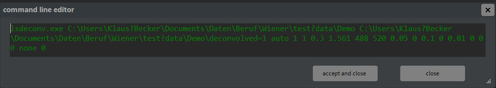
Press the green accept button to save your changes and exit edit mode, or the red button to discard changes. Alternatively, you can modify command lines directly by pressing button A-7, which opens a dialog for editing the command line. The syntax for command lines is explained in chapter 3.
The program only performs a basic plausibility check on direct command line modifications. Incorrect parameters may crash the deconvolution tool (not the GUI), so proceed with caution.
2.2 How to run deconvolution jobs
Once the task list has at least one command line, the start processing button (figure 2.4, item C-1) turns green, indicating readiness to begin deconvolution. Press the start button (figure 2.4, item C1) to start processing the job list from top to bottom. Status information, as well as warnings and error messages that may be generated during deconvolution, are logged in the output window.
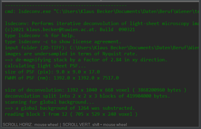
Figure 2.1: The output window displays status information, warnings, and error messages. Output can optionally be logged to a file if configured in the preferences window.
Additional tasks can be added to the job list even while it is processed, but avoid adding a new task just in the moment when the program switches to the next set of input data to prevent occasional crashes.
Deconvolution speed highly depends on input data size and hardware power, ranging from minutes to hours or even days. GPU-based deconvolution is much faster (up to more than 100 times) than CPU mode but requires a compatible Nvidia graphic card (see chapter 1.2 system requirements).
Processing of deconvolution task lists can be scheduled for later, e.g. at night. Click the timer button (figure 2.4, item C-2) to set the start time. The timer button turns red when activated.
Completed deconvolution tasks move to the finalized deconvolutions list located right from the task list (figure 2.4, item A-10). In this list, successful tasks are prefixed with "SUC:", and failed tasks with "ERR:".
Right-click within the task list, finalized tasks list, or output window to access context-related commands (figure 2.5, M1 - M3). TIP: The command repeat deconvolution with changed parameters from menu M2 allows reusing finished command lines, saving much time on re-entering data locations or repeating deconvolutions with another set of parameters.
Structure of a NovoDeblur output folder containing the deconvolved data:
- output folder (standard name: 'deconvolved')
- projections (folder containing preview images)
- xy_mip.tiff (MIP in the xy-direction)
- xz_mip.tiff (MIP in the xz-direction)
- yz_mip.tiff (MIP in the yz-direction)
- xy_mip_orig.tiff (MIP of original data in xy-direction)
- xz_mip_orig.tiff (MIP of original data in xz-direction)
- yz_mip_orig.tiff (MIP of original data in yz-direction)
- decon_info.txt (text file with deconvolution parameters)
- cmdline.info (for internal use when reloading the data into NovoDeblur, do not delete)
- image0001.tiff
- image0002.tiff
- image0003.tiff
...
For each successfully finished deconvolution, a preview image appears in the main window's preview area located at the right side of the main program window (figure 2.2). By default, the preview shows a maximum intensity projection (MIP) in xy-direction. MIPs in the xz and yz directions or slice-by-slice views can also be displayed.
2.3 Visualizing and inspecting your deconvolution results
Double-clicking an image in the preview area opens an enlarged version of the preview image in a result window (chapter 2.4.4). The result window has buttons on the left side for switching between slice-by-slice views or MIP projections along the xy, xz, or yz axes (figure 2.10, items 1-4).
The MIP projections are generated at runtime during deconvolution and stored as tiff-images in the output folder. These images can also be copied and accessed directly, e.g., for use in documents.
In addition, an original window showing the unprocessed data can be displayed parallel to the result window (figure 2.10, item 5, figure 2.11). Any changes of zoom factor, display region or brightness/contrast made in a result window are mirrored in the corresponding original window to ensure an easy comparison of image details before and after deconvolution (figure 2.11, item 4). Further details about reviewing deconvolution results are provided in chapter 2.4.4.
2.4 Description of the main NovoDeblur GUI components
2.4.1 The NovoDeblur GUI window
Launch the NovoDeblur GUI by selecting its entry in the Windows Start menu or by clicking on the desktop icon. The GUI includes a main menu bar at the top, a status bar at the bottom, and the deconvolution window. This chapter explains how to use these elements to define and run deconvolution jobs, as well as how to visualize the results.
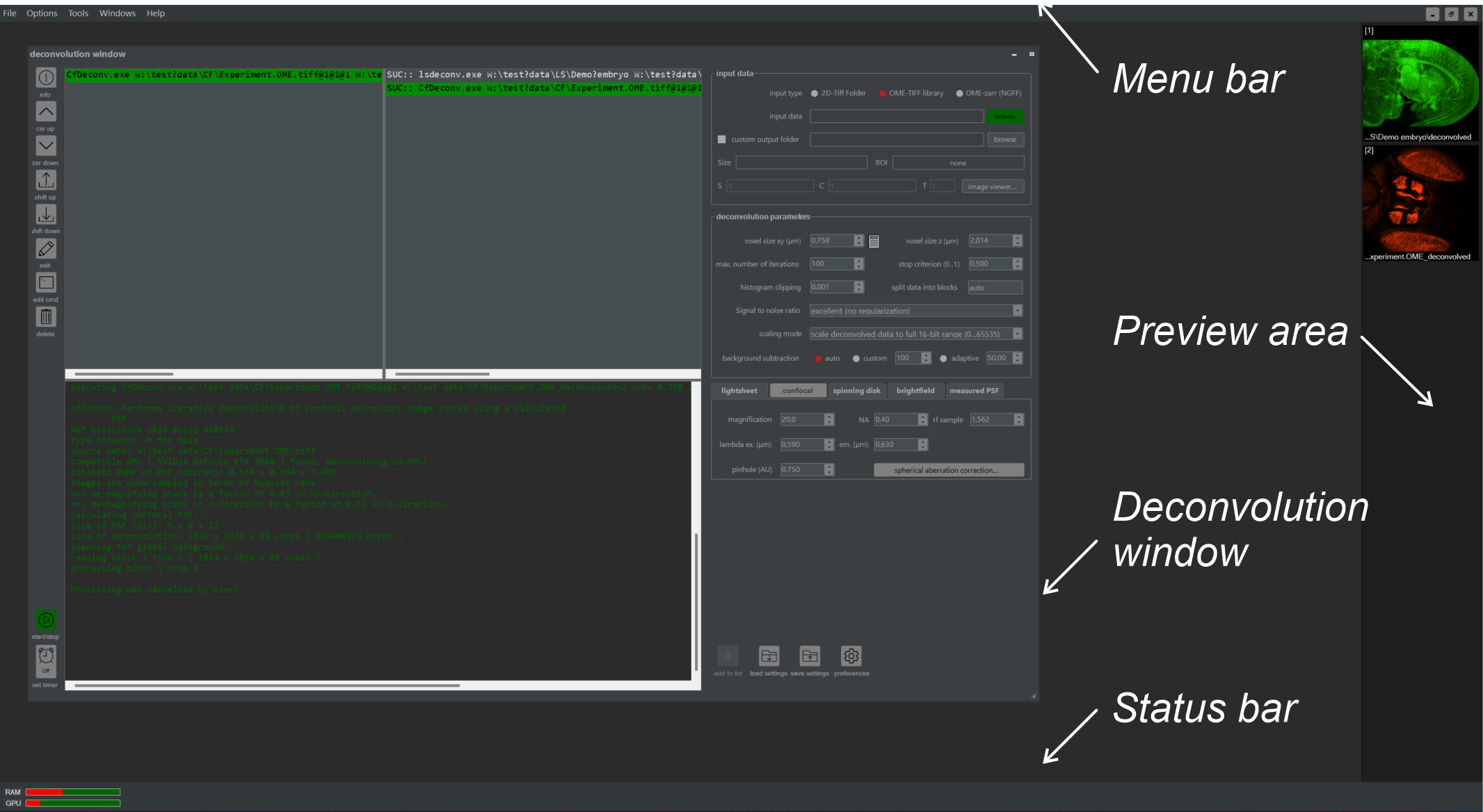
Figure 2.2: Overview of the GUI main window. This includes the deconvolution window, preview area, menu bar, and status bar.
The GUI main window has a menu bar at the top and a status bar at the bottom (figure 2.2). The deconvolution window is used for planning and running new deconvolution tasks.
The pull-down menu bar contains the following entries:
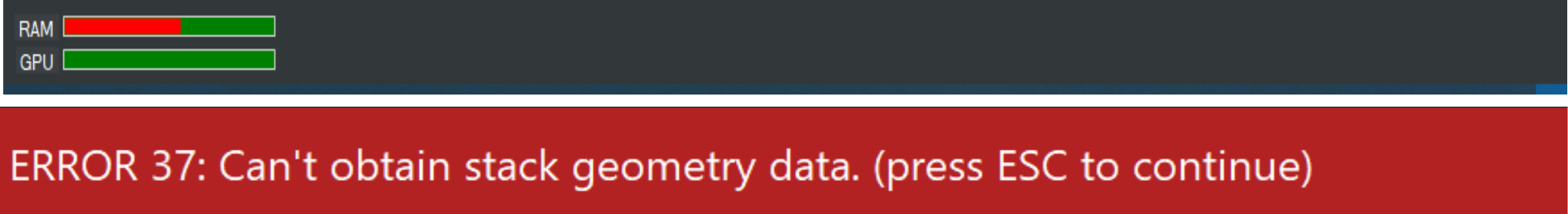
The status bar
The status bar contains graphical indicators for the current usage of RAM and GPU memory. Info, warning, or error messages are displayed here too. These messages disappear automatically after 5 seconds. Alternatively, pressing the ESC key dismisses them immediately.
Figure 2.3: The status bar contains indicator bars showing the currently available RAM and GPU memory (upper image) and also presents warning and error messages (lower image).
2.4.2 The deconvolution window
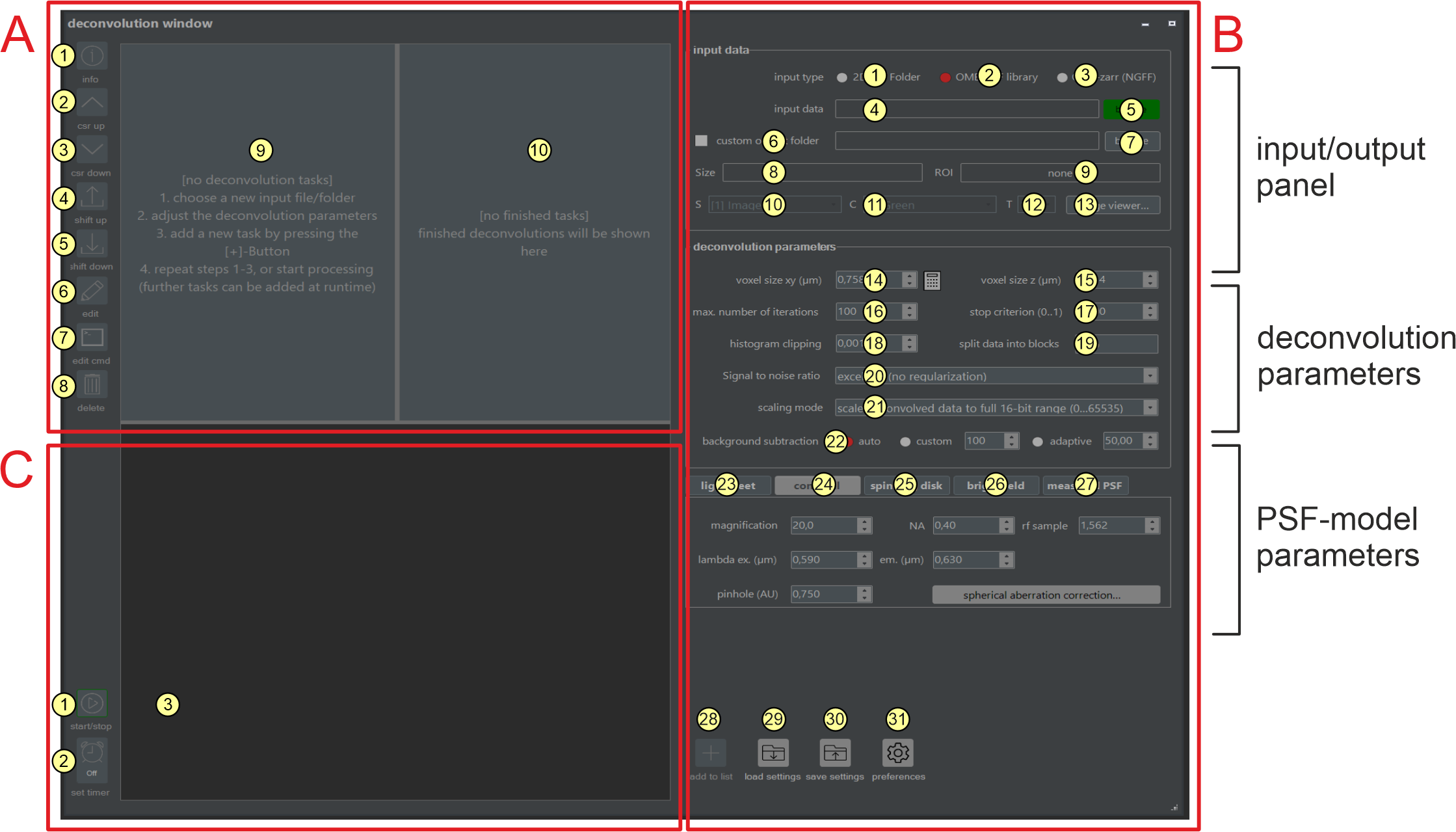
The deconvolution window provides all functions required for planning and executing deconvolution tasks. The window comprises the three main regions: A, B, and C. Scheduled deconvolution tasks (A-9) and already finalized deconvolution tasks (A-10) are shown in Region A. In Region B, parameters for defining a new deconvolution task (e.g., source path, deconvolution type, and microscope setup values) are set. Region C contains buttons for starting and terminating running deconvolution jobs and includes the output window, which shows runtime status messages and contains buttons for starting and terminating running deconvolution jobs (C-1, C-2, C-3).
Figure 2.4 Components of the deconvolution window Most of the functionality provided by the NovoDeblur GUI can be accessed from the deconvolution window. The usage of elements A1 - A10, B1 - B57, C1 - C3, and context menus M1 - M3 is explained below.
- Info: Clicking provides an overview of the deconvolution parameters set for the selected entry in the task window.
- Cursor move up: Clicking shifts the cursor bar one line upwards in the deconvolution task list.
- Cursor Move down: Clicking shifts the cursor bar one line downwards in the deconvolution task list.
- Move command line up: Clicking moves the currently selected command line one line upwards in the deconvolution task list.
- Move command line down: Clicking moves the currently selected command line one line downwards in the task list.
- Edit command line: Clicking switches into edit mode for modifying the deconvolution parameters associated with the selected entry in the deconvolution task list.
- Modify command line: Clicking allows direct editing of the selected command line (use with caution).
- Delete command line: Clicking removes the currently selected entry from the task list.
- Task list: The task list contains scheduled deconvolution tasks. Each entry corresponds to the command line that would be typed when starting this deconvolution from a console window without using the GUI (chapter 3). New entries are added to the task list using the add button.
- Finalized tasks list: This list box shows deconvolution tasks that are already finished. Tasks processed successfully are prefixed with 'SUC:'. Tasks that stopped with an error are prefixed with 'ERR:'.
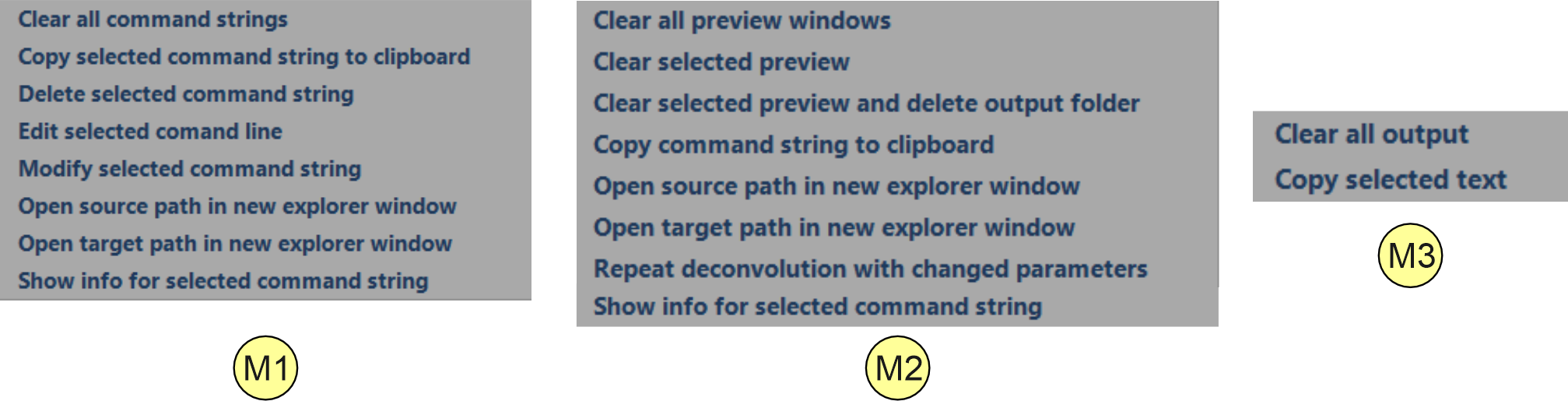
Context Menues avaiable by right mouse click within the task lists
Figure 2.5: Context menues that opens up by right click if the mouse curser is within in the the task list control (M1), the 'finished tasks list' control (M2) or within the output window area (M3). For a description of the different menu items see below.
Pull-down menu M1 (see figure 2.5)
Menu opens via right-click if the mouse cursor is in the 'task list control' (A-9).
- Clear all command strings: Deletes all entries from the task list (A-9).
- Copy selected command sine to clipboard: Copies the currently selected task list entry (A-9) to the clipboard.
- Delete selected command string: Same functionality as button (A-8).
- edit selected command line: Same functionality as button A-6.
- Modify selected command string: Same functionality as button (A-7).
- Open source path in new explorer window: Opens the raw data location defined in the currently selected command line in a new explorer window.
- Open target path in new explorer window: Opens the target folder defined in the currently selected command line in a new explorer window.
- Show info for selected command string (same functionality as button A-1).
Pull-down menu M2 (see figure 2.5).
Menu opens via right-click if the mouse cursor is within the 'finished tasks control' (A-10).
- Clear all preview windows: Removes all result windows that are currently open or iconified.
- Clear selected preview: Closes the active result window.
- Clear selected preview and delete output folder: Removes the active result window and deletes the associated result data. A confirmation dialog box appears before deleting any files.
- Copy command string to clipboard: Copies the currently selected task list entry (A-10) to the clipboard
- Open source path in new explorer window: Opens the source folder specified in the selected command line in a new explorer window.
- Open target path in new explorer window: Opens the target folder specified in the selected command line in a new explorer window.
- Repeat deconvolution wiith changed parameters: Copies the command line currently highlighted in the finalized deconvolutions list back to the deconvolution task list (A-9). If the output folder name already exists, a unique name is suggested by adding a numeric postfix (e.g., test1, or test2) and activates the edit mode for modifying the deconvolution parameters (also see figure 2.4, item A-6). This approach avoids starting from scratch when you want to repeat a deconvolution with an alternative set of parameters.
- Show info for selected command string
Pull-down menu M3 (see figure 2.5).
opens after a right-click within the output window (C-3).
- Clear all output: Deletes all text from the output window.
- Copy selected text: Copies the selected text to the clipboard.
Controls for specifying the deconvolution parameters (figure 2.4 region B)
- Input type 2D-tiff Folder: Check this radio button to process a numerically ordered series of 2D-tiff images (16-bit or 32-bit) located in one folder. The image file names must have trailing numbers (e.g., tiff0001.tif, tiff0002.tif) of equal length, padded with leading zeros.
- Input type OME-tiff library: This radio button needs to be checked for processing multidimensional OME-tiff libraries. OME-tiff libraries can contain multiple image series (S) with up to 5 dimensions each (C: color channel, T: time point, X: image width, Y: image height, Z: number of images in the stack). OME-tiff supports an extensive set of metadata and is supported by many manufacturers of microscopes and image processing software. For more informations about the OME-tiff specification please have a look here.
- Input type OME-zarr (NGFF). NGFF (Next Generation File Format) is an image format specifically designed for the efficient storage of microscopy data in the cloud. Given that the format is relatively new, it is still undergoing significant development.
- Input path info: Read-only text field showing the currently selected input path.
- Open source data: Clicking opens a file or folder selector box (depending on the selected input type, see B-1 - B-3) for specifying a new source data location.
- Select custom folder: Select Custom Folder: If checked, a custom output folder can be specified after pressing the path selector button (B-7). Otherwise, the deconvolved data are written to a default folder named “deconvolved-m” that is generated within the source data folder. If required, the index m will be automatically appended to the folder name to avoid a conflict with an already existing folder name.
- Output path selector: Clicking on the button opens a folder selection box to specify a custom output location. This button is only enabled if check box B-5 is checked.
- Size info: Displays the dimensions of the currently selected input image stack (x, y, z order) if there is any.
- ROI info: Shows the coordinates of a region of interest (ROI) if one is specified in the image inspector.
- Series info (S): Displays the index of the currently selected image stack. This is only relevant for OME-tiff image libraries containing multiple image stacks.
- Color channel info (C): Displays the channel index of the currently selected color channel. This is only relevant for OME-tiff image libraries containing multiple color channels.
- Time point info (T): Displays the channel index of the currently selected time slice. This is only relevant for OME-tiff image libraries containing multiple image stacks that were recorded at different points in time.
- image inspector: Clicking the button opens the image inspector. The image inspector allows defining a ROI and selecting series (S), color channels (C), and time slices (T) from a 4 or 5-dimensional OME-tiff library.
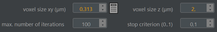
- Voxel size xy: The physical size of one voxel in xy-direction. This value equals the size of a camera pixel that is back-projected into the image plane (vxy = pxy / Mtot, where vxy is the voxel size, pxy is the physical size of a camera pixel and Mtot is the total magnification of the microscope). Clicking on the calculator icon to the right of the input field opens a tool for estimating the correct voxel size. This calculator requires the magnification of the objective, the post-magnification of the microscope (tube lens), and the camera chip geometry data as inputs. These values can typically be found in the manuals provided by the microscope and camera manufacturers. Alternatively, the xy-voxel size can be determined experimentally using an object micrometer. For low magnification objectives (e.g., 2x or 4x), it can also be measured by imaging a small sheet of squared paper with known square dimensions as a reference.
- Voxel size z: The dimension of a single voxel in the z-dimension (microns). This describes the distance between neighboring image planes in the input stack.
- Max. iterations: Specifies the maximum number of deconvolution rounds. The iterative deconvolution process terminates when this value is reached or if the quality measure calculated during each iteration step becomes lower than the predefined stop criterion (B-18).
- Stop criterion: Specifies a numeric criterion for terminating the deconvolution process. At the end of each iteration, the program calculates a quality indicator measuring the achieved gain in image quality. If this value becomes smaller than the stop criterion, the iteration loop stops. Increasing the number of iterations by lowering the stop criterion can improve the deconvolution results but increases the processing time, as more iterations will be performed. If the chosen number of iterations is too high, typical artifacts (so-called ringing artifacts) can occur in the deconvolved data. These artifacts are characterized by ring-shaped structures mainly present along strong intensity transitions within the images. If you lower the stop criterion, you may also need to increase the max. iterations value (B-17) to prevent it from becoming the limiting factor. The current iteration number and the value of the quality indicator are printed to the output window (C-3) at each iteration round.
- Histogram clipping value: This sets the amount of clipping at the right side of the histogram in percent. For example a value of 0.01% indicates that the histogram of the deconvolved stack gets clipped at its 99.99% percentile. All higher intensities values are clipped to this value. After clipping the light intensities are linearly rescaled to the the full 16-bit range (0..65535) if this feature is set in the scaling mode combo box (B-21). Deconvolved 32-bit images are always rescaled to the intensity range of the raw data if the scaling is active.
- Split data into blocks: This setting determines how large data sets are divided into blocks. The recommended setting is "auto". In this mode, the optimal block splitting is determined automatically using the following algorithm: Starting with the original data set as the first data block, all blocks are repeatedly split in half along their longest edge until all resulting blocks are small enough to be deconvolved in a single pass. The maximum number of voxels a data block can have to be deconvolved in a single pass is specified in the preferences dialog window under "memory settings". This value is specified as a percentage of the total available RAM and GPU memory in your computer. Alternatively, block generation can be controlled manually by entering a string in the format "k x n x m", where k, n, and m represent the number of splits performed along the x, y, and z directions, respectively. For example, entering the string "2x3x4" would split the original data into a total of 24 blocks, which are then deconvolved in sequence and stitched together afterward.
- Signal to noise ratio: Here, an estimate for the signal to noise ratio of the recorded images can be entered. Options include excellent (0.0), good (0.01), average (0.025), poor (0.05), very poor (0.075), and custom. The first two options are suitable for light sheet microscopy, which generally has a very good S/N ratio. Other options are more useful for confocal microscopy data, which are often noisier. For finer quantification, the custom option allows specifying a numeric value q between 0 and 0.5. NovoDeblur uses flux-preserving regularization to limit noise amplification during deconvolution. The value of q should be sufficiently high to limit noise amplification but low enough to avoid unwanted blurring. Example figure 6 shows a comparison between deconvolutions of the same dataset without and with regularization. The deconvolution without regularization shows noticeable noise amplification, while the deconvolution with regularization shows improved quality.
- Scaling mode: Sets the scaling method for output data. Choosing scale deconvolved data to full 16-bit range scales the intensities of the deconvolved images to the full 16-bit range (0 to 65535), i.e., the lowest intensity value in the entire image stack becomes 0 and the highest value becomes 216 - 1 = 65535. Scaling of 32-bit images is always done in a way that the highest intensity value matches the maximum intensity value in the raw data. Selecting apply no scaling means that no output scaling is performed at all. Choose this option if you need to perform a quantitative comparison of intensity values across multiple data sets or if you plan to stitch multiple deconvolved data sets together later on.
- Background removal parameters: The options for image background removal before deconvolution are available: auto, custom and adaptive (figure 2.6).

Figure 2.6: Possible options for background subtraction are auto (1), custom (2), or adaptive (3).
Choose auto (1) for automatically determining and subtracting the minimal background value present in the stack of raw data . Use custom (2) if you want to subtract a constant user-defined intensity offset from the value of each voxel (any negative values are clipped to zero). Use adaptive (3) to perform adaptive background subtraction using a rolling ball filtering approach. The filter is sequentially applied along all three data planes of the stack, i.e., xy, xz, and yz. The scaling of the filter radius r is always in µm; for example, entering a value of 75 µm applies a spherical structuring element of 150 µm diameter. Small values for the radius r will result in a higher amount of background subtraction than larger values.
- Light sheet tab: Select this tab to deconvolve light sheet microscopy stacks using a computed PSF.
- Confocal tab: Select this tab to deconvolve confocal microscopy stacks using a calculated PSF. For the meaning of the different input fields please see under "Deconvolution mode dependent options" below.
- Confocal tab: Select this tab to deconvolve confocal microscopy stacks using a calculated PSF. For the meaning of the different input fields please see below.
- Brightfield tab: Select this tab to deconvolve confocal microscopy stacks using a calculated PSF.For the meaning of the different input fields please see under "Deconvolution mode dependent options" below.
- Measured PSF tab: Select this tab to deconvolve image stacks using a measured PSF.For the meaning of the different input fields please see under "Deconvolution mode dependent options" below.
- Add task button: Clicking this button appends a new command string to the task list (A-9) using the source data and deconvolution parameters currently specified in region B of the deconvolution window. After all required fields have been populated, the color of the add task button changes to green, indicating that a new command string can be generated.
- Load parameter set: Use this button to reload a previously saved set of deconvolution parameters. Clicking this button opens a file selector box to choose a parameter file. Parameter files usually have the file extension .AppSettings.
- Save parameter set: Use this button to store the current deconvolution parameters (B14 - B38) for later use. Clicking opens a file selector box for selecting a file name. If missing the extension .AppSettings is added automatically.
- Preferences dialog window: Clicking the buttun opens the preferences dialog for making various presets controlling the program's behavior.
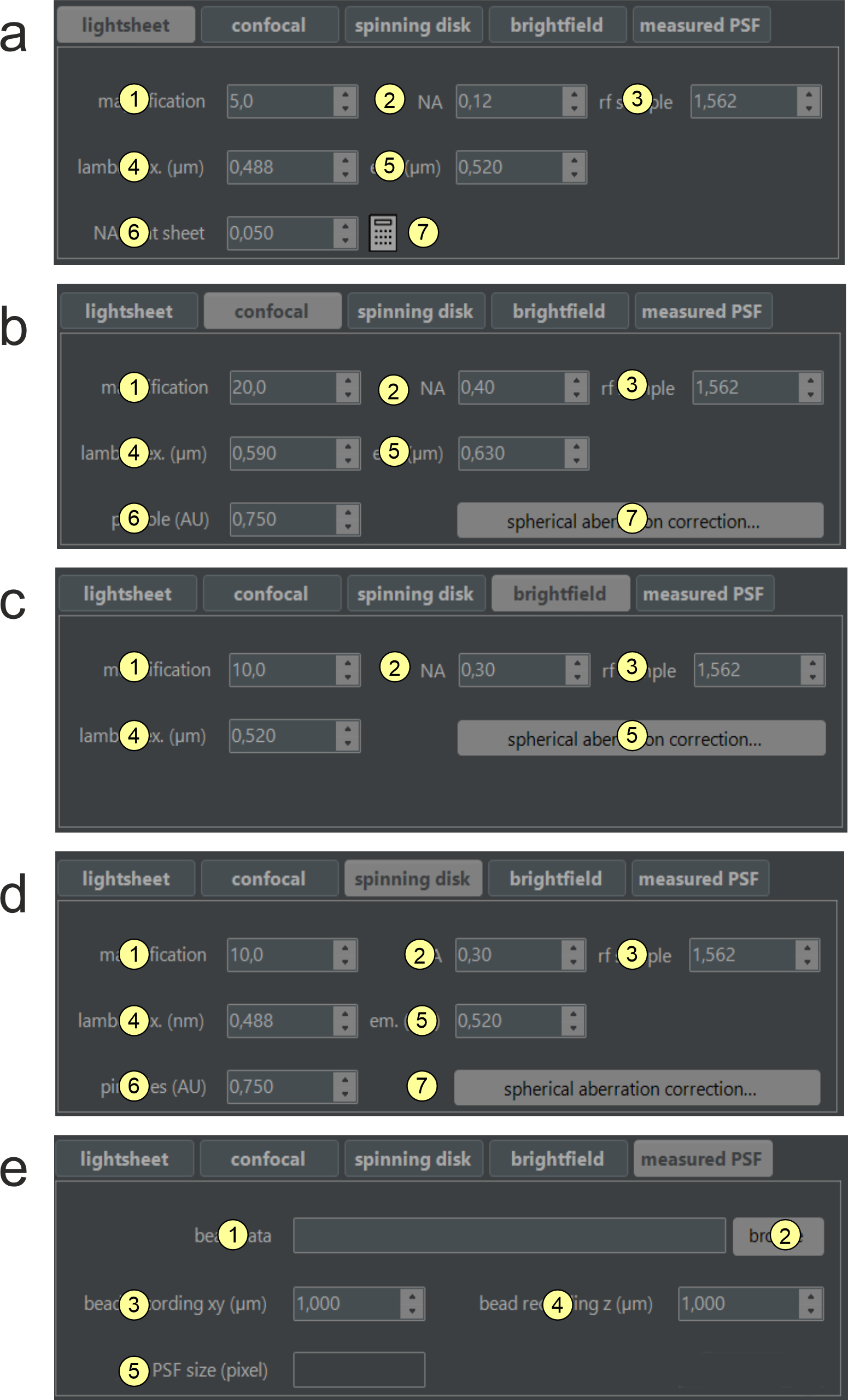
Deconvolution mode specific TAB-controls
This section describes the input controls that are located within the tab-windows (B-23 - B-27) within region B of the deconvolution window (figure 2.4).
Figure 2.7: Deconvolution mode dependent options. Novodeblur supports deconving image stacks obtained with different types of microscopy as a) light sheet microscopy, b) confocal microscopy, c) spinning disk confocal microscopy, d) brightfield and e) deconvolution using a measured PSF. For the options a - d a calculated PSF is applied that is specific for the respective imaging type. If you have a mesaured PSF choose option e regardless of the type of your microscope. For the meaning of the parameters in the 5 different tabs please have a look at the explaniations below.
a) Light sheet microscopy tab (figure 2.7 a)
- Magnification: Enter the magnification of the objective you use for recording here.
- NA: Enter the numerical aperture of the objective used for recording here. Values must range from 0.1 to 1.4.
- rf sample: Enter the refractive index of the medium in which the sample is immersed during recording.
- lambda ex. (µm): Enter the laser wavelength used for fluorescence excitation.
- lambda em. (µm): Enter the peak wavelength of the fluorescence emission spectrum.
- NA Light sheet: Enter the numerical aperture (NA) of the light sheet generator here. For a basic light sheet microscope with a single cylindrical lens and a slit aperture in front of it, the NA can be calculated using the calculator tool (B-7). Otherwise, find the NA in the light sheet microscope manual. A higher NA results in a thinner beam waist at the focus line but a smaller Rayleigh range. Once optimized, this parameter usually remains constant for a given setup. If unavailable, estimate 0.05 and vary between 0.01 and 0.1 in steps of 0.01 to find the best value for your setup.
- Light sheet NA calculator: This tool calculates the NA for a basic light sheet generator form the focal length of the cylinder lens and the width of the slit aperture located in front of it.
b, c) Confocal and spinning disk microscopy tabs (figure 2.7 b and d)
- Magnification: Enter the magnification of the objective you use for recording here
- NA: Enter the numerical aperture of the objective used for recording here. Values must range from 0.1 to 1.4.
- rf sample: Enter the refractive index of the medium in which the sample is immersed during recording.
- lambda ex. (µm): Enter the laser wavelength used for fluorescence excitation.
- lambda em. (µm): Enter the peak wavelength of the fluorescence emission spectrum.
- pinhole (AU): Please enter the normalized diameter of the confocal pinhole of your microscope in airy disk units (AU). If the back-projected pinhole diameter is provided by your microscope manufacturer, the normalized pinhole diameter (AU) can be calculated using the relation AU = (d x NA) / (1.22 x λ), where d is the back-projected pinhole diameter in microns, NA is the numerical aperture of the objective, and λ is the fluorescence emission wavelength. If only the physical pinhole size is known, the back-projected pinhole diameter d can be calculated using the relation d = d' / (Mobj x M0), where d' is the physical pinhole diameter, Mobj is the objective magnification, and M0 is the intrinsic magnification factor of the microscope (e.g. magnification of the tube lens).
- Spherical aberation correction: NovoDeblur can optionally consider refractive index mismatches between the different optical materials the light that is collected by the objective has to pass when calculating a PSF.
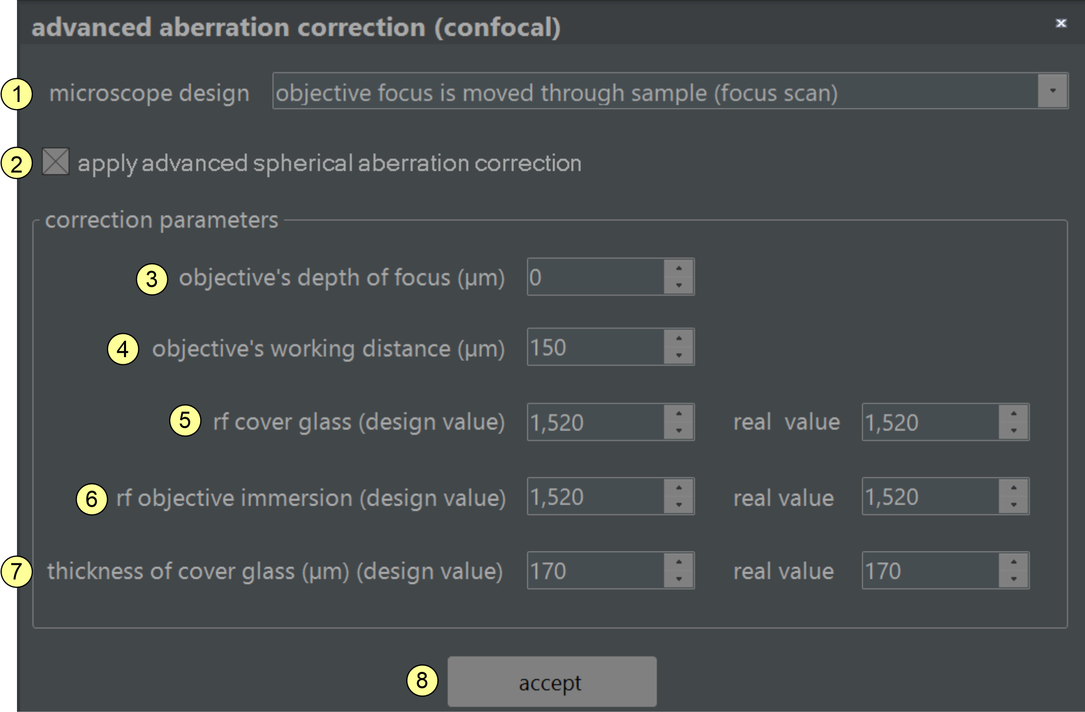
Figure 2.8 Spherical aberration correction: NovoDeblur can account for spherical aberration caused by moderate refractive index mismatches between the various materials through which the light from the sample passes (e.g., embedding medium, cover glass, immersion oil, objective). To achieve this, NovoDeblur needs to know the design specifications of the objective as well as the actual values used in microscopy. Please refer to the text box below for a description of the required parameters.
Spherical abberration correction window (figure 2.8):
- This option specifies the design type of the microscope: choose "focus scan" if the objective changes its distance relative to the object carrier and sample while scanning along the z-axis. In this mode, the lengths of the pathways the light beam travels through different media (e.g., air and glass) change during recording. In the second mode, "sample scan" the objective is typically equipped with a dipping cone that dives into a bath solution filled with a clearing medium. During scanning, the sample container is shifted along the z-axis. Since the dipping cone always remains submerged in the liquid, the optical path differences remain constant during recording.
- Please mark this checkbox to use spherical aberration correction during deconvolution. Uncheck it otherwise.
- Specify the depth you are looking into the immersion medium, measured from the lower surface of the cover glass.
- Specify the working distance (WD) of the objective. You usually find this parameter engraved on the objective.
- Enter the refractive index of the cover glass here. Typically, it is 1.52.
- Specify the refractive index of the medium in which the front lens of the objective is immersed. The refractive indices of the immersion medium and the sample are assumed to be identical.
- Specify the thickness of the cover glass here. A standard value is 0.17 mm. Enter zero if you don't use a cover glass.
- Accept changes and close dialog window.
d) Brightfield microscopy tab (figure 2.7 c)
- Magnification: Please enter the magnification of the objective here
- NA objective: Please enter the numerical aperture of the objective used for recording here. Values must range from 0.1 to 1.4.
- Refractive index: please enter the refractive index of the medium in which the sample is immersed during recording. Sample and immersion medium are assumed to have the same refractive index
- Excitation wavelength (nm): Please enter the laser wavelength used for fluorescence excitation.
- Spherical abberation correction: clicking opens a window for setting the parameters for optional corection of spherical aberration. For an explanation of the parametes please have a look at figure 2.8 and the relatred text box below.
- PSF path info: Shows the path of the folder containing the measured PSF data (read-only field).
- PSF path selector: Clicking opens a folder selector box to choose the folder containing the measured PSF data. The PSF must be stored as a series of numbered 16-bit grayscale tiff images of square shape. All images must be square and of the same size, with file names having numerical endings of equal length (e.g., psf00001.tif, psf00002.tif).
- PSF voxel size xy: The voxel size of the PSF in the XY-direction (microns). If this value differs from deltaXY (14), the PSF is interpolated to match the source data's sampling.
- PSF voxel size z: The voxel size of the PSF in the Z-direction (microns). If this value differs from deltaZ (B-16), the PSF is interpolated to match the source data's sampling rate.
- Original PSF size (pixel): The lateral size of the measured PSF in pixels (read-only field).
Buttons for running deconvolution tasks (figure 2.4 region C)
- Start/stop processing button: Clicking starts processing the task list (A-9). The background color of the button is green if the task list is ready to be processed (i.e., it is not empty and no deconvolutions are running). A red background indicates an active deconvolution task. Clicking opens a dialog box asking whether to terminate it. Adding new tasks to the job list is possible even while it is being processed.
- Set timer button: This function allows running the job list at a later time. This option is available if there is at least one entry in the task list. Clicking the clock symbol sets the preferred starting hour. If activated, the timer button background changes to red.
- Output window: All output generated by the NovoDeblur is monitored in this window. The output window content can be logged to a file by activating the option in the preferences window.
2.4.3 The image inspector
If the respective option is enabled in the preferences dialog window (figure 2.13, item (7)), the image inspector opens automatically after choosing an input dataset. Otherwise, it can be opened by clicking the image inspector button (figure 2.4, item B-13).
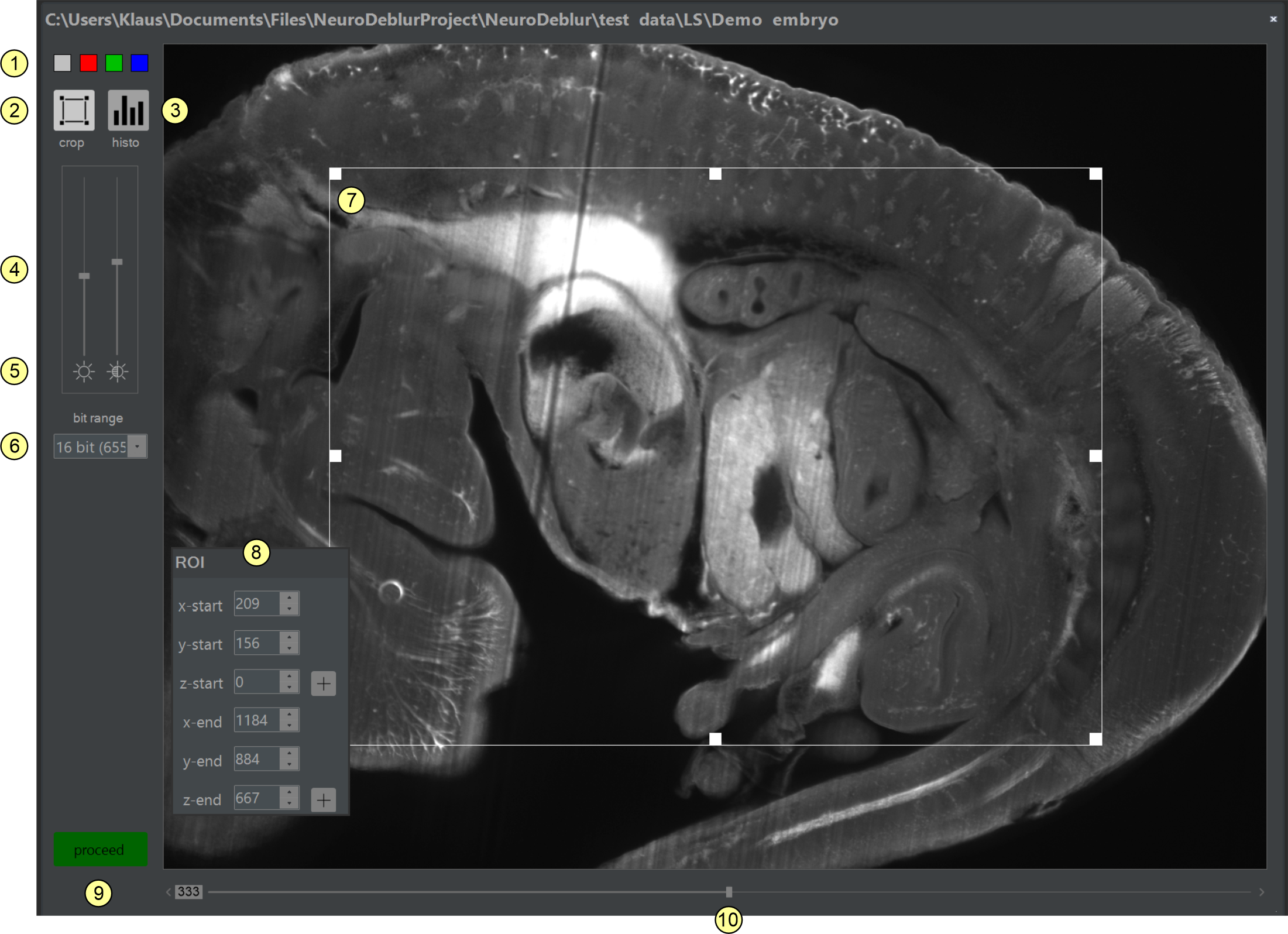
Figure 2.9: The image inspector. The image inspector allows selecting a distinct color channel or time slice from multi-dimensional image libraries and cropping an input image stack before deconvolution.
Elements of the image inspector (figure 2.9)
- Color map selector: Clicking on one of the four colored squares sets the display color of the preview window.
- ROI selection tool: Clicking shows/hides the ROI selector (7)
- Histogram tool: Opens the tool for calculating a 3D-histogram of the entire stack or the currently selected ROI, if any.
- Brightness and contrast slider: Adjusts the brightness of the preview image. Changes affect the screen representation but not the underlying data.
- Reset brightness/contrast buttons: Clicking on the two icons resets the brightness or contrast (4) to their default values (zero).
- Dynamic range adjustment: Here, you can specify the number of valid bits used for displaying tif-images. For example, for images recorded with a camera with 4096 intensity values (= 12 bit) that are encoded as 16-bit tiff files, selecting 12-bit will normally provide the best screen representation. For 32-bit images, they are automatically scaled to the highest occurring intensity value, so this setting is not shown for 32-bit images.
- ROI selector: Dragging or resizing the rectangular frame sets the x and y coordinates of an ROI graphically. Alternatively, the coordinate values can be entered numerically in the ROI coordinates window (1). The z-extensions of an ROI can only be entered in the ROI coordinates window (8).
- ROI coordinates window: If the ROI selector tool (7) is active, the x, y, and z coordinates of an ROI can be specified by entering the coordinates instead of using the mouse. The z-coordinates defining the z-dimension can only be defined here. Clicking the + and - buttons right of the numerical input fields labeled z-start and z-end pastes in the number of the currently selected slice.
- Clicking this button closes the image inspector window.
- Z-position slider: Allows selecting the image from a raw data stack that is displayed. Numbering starts from zero.
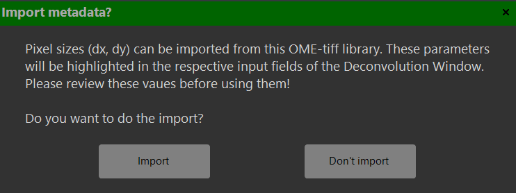
Import of metadata from OME-tiff libraries:
OME-tiff libraries can contain descriptive metadata (e.g., specifying voxel size or objective NA). After inporting these data a dialog window asks whether to import some of these metadata. The current version only supports importing voxel sizes and and the names of the channels comprised in the library.
Press 'Yes' to confirm the import or 'No' to continue without importing. Imported values are highlighted in orange in the deconvolution window.
Imported values are tintet in orange color, which is removed after editing these values. Please review the imported parameters for plausibility before running the deconvolution.
Once the image inspector is closed, the color of the add button (figure 2.4, item B-39) turns to green, indicating that all input values were validated asuccesfully, and a new entry is added to the task list. Possible errors messages are displayed in the main window status bar.
2.4.4 The result windows
After deconvolution finishes, a preview image visualizing the deconvolution result is appended to the preview area of the main program window (figure 2.2). The preview window either shows a single slice or a maximum intensity projection (MIP) of the entire stack, depending on the respective setting in the preferences window. Double-clicking the preview image or choosing magnify image from the context menu activated by a right mouse click opens a result window (figure 2.10). Here, the deconvolved data can be inspected by zooming and panning with the mouse. An image stack can be visualized slide by slide or via MIP projections along the xy, xz, or yz planes. To ease comparisons between raw and deconvolved data, a second display window that optionally synchronizes automatically with the result window can be displayed (figure 2.11).
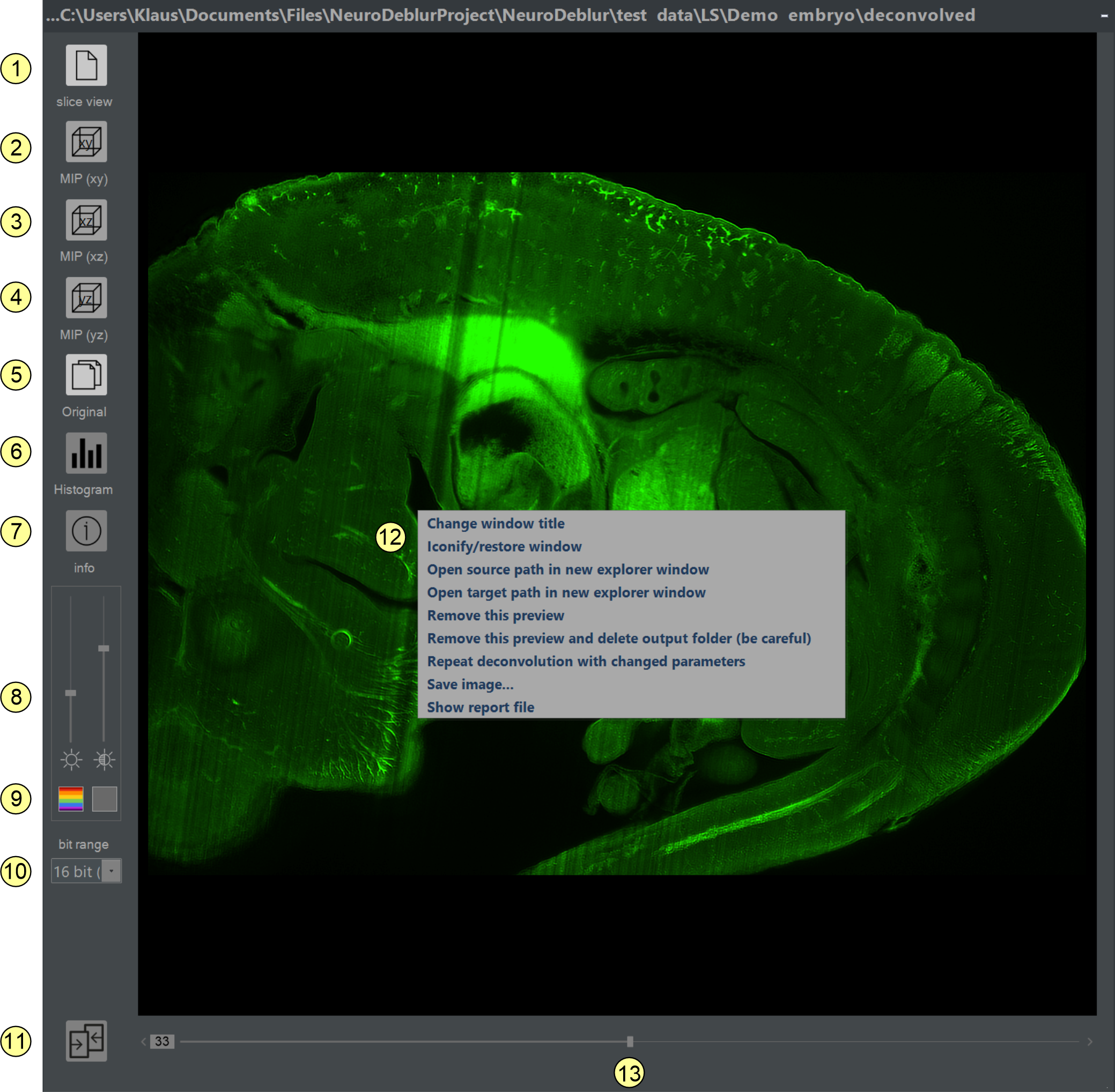
Figure 2.10: Double-clicking a preview image in the main window (figure 2.2) opens a result window for detailed inspection of deconvolution results.
Elements of the result window (figure 2.10)
- Single Slice View: Click to scroll through deconvolved data slice by slice. If selected, a scrollbar (12) appears at the bottom of the window for scrolling through the images.
- MIP projection (xy-view): Click to display a maximum intensity projection along the z-axis of the deconvolved stack.
- MIP projection (xz-view): Click to display a maximum intensity projection along the y-axis of the deconvolved stack.
- MIP projection (yz-view): Click to display a maximum intensity projection along the x-axis of the deconvolved stack.
- Show original button: Clicking opens an original display Window for comparing the raw data and the deconvolved data (figure 2.11). The content of the original display window synchronizes automatically with the content of the result window if the sync geometry check box is checked (figure 2.11, item-4). See here for a more detailed description about the different components of the original display window.
- Histogram: This options allows to plot a 3D-Histogram of the underlying stack of raw data.
- Show info button: Clicking opens a text window displaying the content of the info file generated for each deconvolution task (figure 2.12).
- Contrast/brightness slider: Adjusts the contrast and brightness of the displayed image. Changes only affect the screen representation.
- Color selector: Renders the image in gray levels (left button) or using a luminance table (LUT) matching the emission wavelength specified for this deconvolution.
- Dynamic range selector: This selection box appears only for 16-bit tiff-images. The number of 'used' camera bits (e.g., 11-bit = 2048 to 16-bit = 65536) can be set here. If the imaging software encodes intensity values from 0 to 4095 (=2^12-1 = 12 bits) into 16-bit tiff-images, choose 12-bit for the best screen representation. This setting is not available for 32-bit images, which are always scaled to the maximum intensity value.
- Make same size tool: When working with multiple 'result windows' in parallel, synchronizing their sizes or displayed regions can be convenient. Click the make same size icon at the left-bottom of the result preview window. The mouse cursor changes to a hand symbol. Click a second result window to make its zoom factor and shape equal to the first window.
- A right mouse ckick within the result window opens a context menu offering different options for making
- Select slice scrollbar: If single slice view (1) is activated, this slider scrolls through the entire stack.
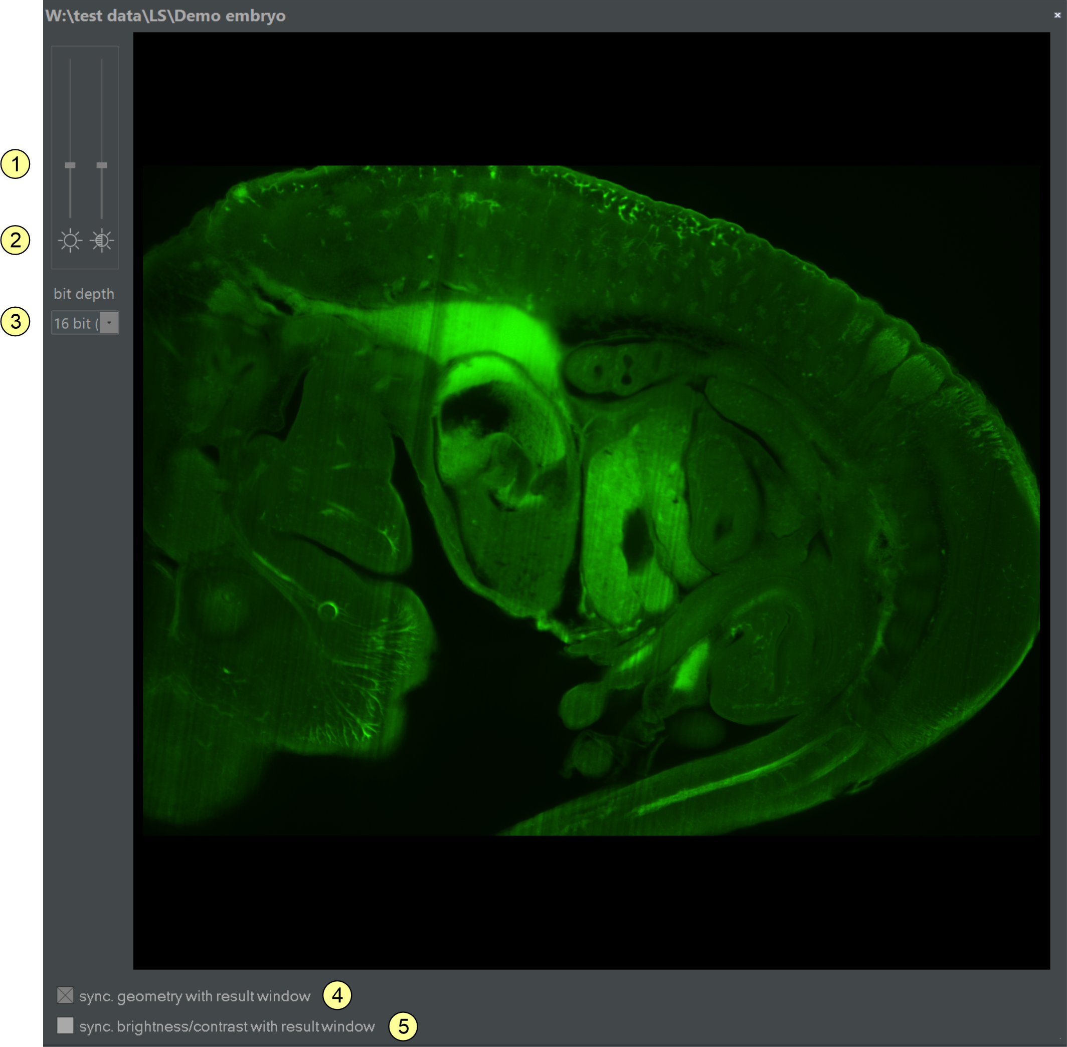
Figure 2.11: Clicking the show original button (5) in a result window opens an 'original display window' like this, showing the related original data. The content and shape of this window automatically synchronize with the result window in focus. This synchronization feature can be toggled on or off via the sync checkbox (4).
Elements of the original display window (figure 2.11)
- Contrast/brightness Slider: Adjusts the contrast and brightness of the displayed image. Changes only affect the screen representation.
- Reset brightness/contrast buttons: Clicking on the buttons below the sliders resets brightness or contrast to their default values (zero).
- Dynamic range selector: This selection box appears only for 16-bit tiff-images. The number of 'used' camera bits (e.g., 11-bit = 2048 to 16-bit = 65536) can be set here. If the imaging software encodes intensity values from 0 to 4095 (=2^12-1 = 12 bits) into 16-bit tiff-images, choose 12-bit for the best screen representation. This setting is not available for 32-bit images, which are always scaled to the maximum intensity value.
- If checked the displayed region in the Original Display Window is synchronized with the respective image region in the Result Viewer Window. Shiftting or zoming the result image using the mouse causes the same change in the Original Display Window (but not vice versa).
- If checked contrast and brightness of the Original Display Window are synchronized with the Result Viewer Window. Changes of contrast or birghtness made for the Result Viewer Window are also applied to the Original Display Window (but not vice versa).
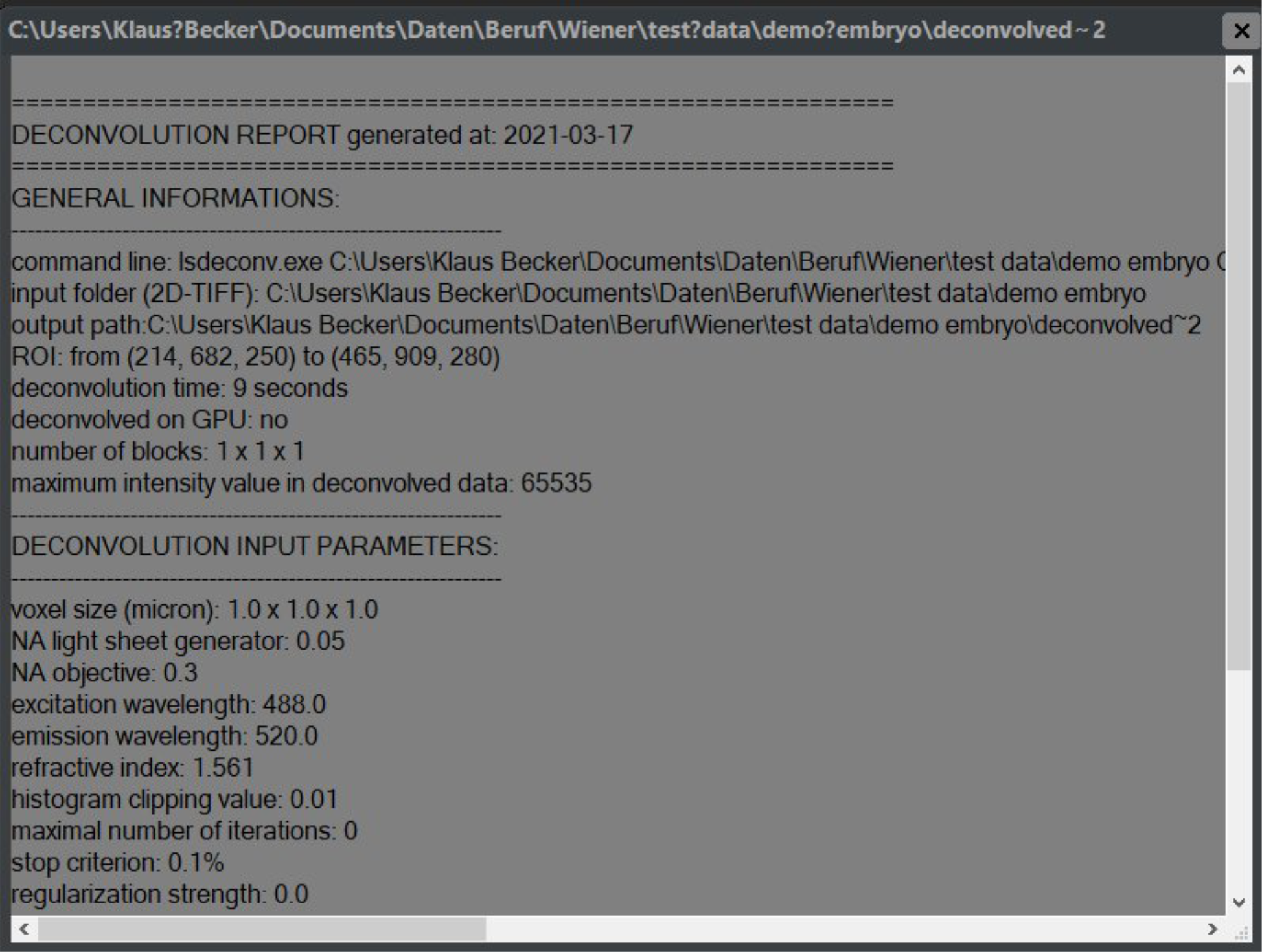
The report file window (figure 2.12)
Figure 2.12: The Report file window displays a detailed report for each finished deconvolution task, comprising an overview of the applied decopnvolution paramerters, file pathes, date and required time and others.
For each succcessfull deconvolution a report file named "decon_info.txt" is generated and stored in the folder structure comprising the according data (figure 2.12). Clicking the show info button located at the lift side of a result window (figure 2.10, item 7) opens this file in a new text window.
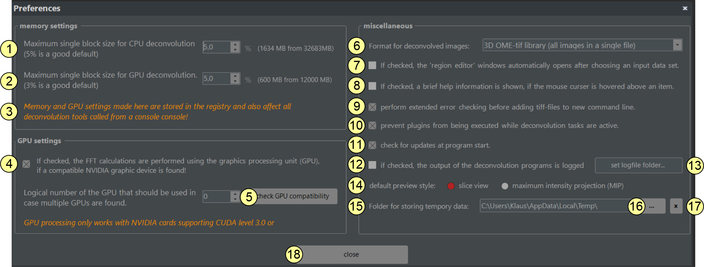
2.4.5 The preferences dialog window
The preferences window is used to set defaults controlling the properties of the deconvolution tools and GUI. Some presets are stored in the registry and will be applied if the tools are directly invoked from a console window (see chapter 2.4.6 for details).
Figure 2.13: The Preferences Window. Different settings modifying the program's behavior are made here. Changes become active immediately and are restored at the next program start.
- Maximal memory usage for CPU-based deconvolution: This input field sets the maximal size of a data block that can be deconvolved in one pass. The value is provided as a percent fraction of the available RAM. For example, 5% of 16 GB RAM allows an 800 MB data block. Larger stacks are split, deconvolved sequentially, and stitched later. A value of 5% is usually good for most computers but can be increased on workstations with more RAM (e.g., 64 GB or 128 GB). Setting the value too high may cause 'out of memory' errors. This setting is stored in the Windows registry and applies to all later deconvolutions, whether started from the GUI or a command window.
- Maximal memory usage for GPU-based deconvolution: This control sets the maximal size of a data block for GPU-based deconvolution, provided as a percent fraction of the available GPU memory. For example, 5% of 8 GB RAM allows a 400 MB data block. Larger stacks are split, deconvolved sequentially, and stitched later. Increasing this value can speed up deconvolution, but setting it too high may cause 'out of memory' errors. This setting is stored in the Windows registry and applies to all following deconvolutions, whether started from the GUI or a command window.
- Logical GPU number input field: Most computers have a single GPU assigned to logical GPU number 0. For multiple GPUs, these are addressed as GPU-0, GPU-1, etc. The desired GPU can be activated using this field. Only compatible Nvidia GPUs are considered.
- FFT calculation mode check box: If activated, the GPU is used for FFT calculations instead of the CPU. GPU-based calculation is typically over 10 times faster than CPU-based, depending on CPU cores and GPU power. An Nvidia compatible GPU with at least CUDA level 3.0 and sufficient memory is required. If no suitable GPU is found, CPU-based mode is used and a message is shown in the output window (figure 2.4, item C-3).
- GPU compatibility check button: Clicking this button performs a compatibility test to check if the active GPU (3) is suitable for GPU-based deconvolution. If successful, the option to activate the faster GPU-based FFT calculation mode (5) is offered.
- Here you can select whether the deconvolved data are stored as a series of seperate, numbered 2D tiff-files (default) or as a 3D OME-tiff library comprised in a single file.
- Auto open image inspector check box: If checked, the image inspector window opens automatically after defining a new input stack. Otherwise, it must be opened explicitly by clicking the image inspector button (figure 2.4, item B-13).
- Show tool tip help check box: If checked, a brief help text appears when hovering over most control elements (e.g., buttons, check boxes, sub-windows). This option can be turned off after gaining experience with the program.
- Perform extended error checking: If checked, all tiff-files in a selected input folder are checked for read errors and format/header issues. Errors prompt a warning message.
- Prevent plugins from executing while deconvolution tasks are running: This default setting prevents plugin use (e.g., for CLAHE or image destriping) during deconvolution. This safe mode can be disabled on machines with enough memory or when deconvolving in GPU mode (which requires less RAM), allowing plugin use during background deconvolution. High memory consumption can cause system non-responsiveness.
- Search for updates at program start: If enabled, NovoDeblur checks for newer software versions at each start and informs via popup message box.
- Enable logging check box: If checked, all text written to the output window (figure 2.4, item C-3) is saved to a log file. Each new session generates a separate log file, indicated by the suffix '*.log' and comprising date and time of generation. By default, they are stored in a folder named NovoDeblur-logfiles on the desktop. An alternative location can be specified using the set log file folder location button (13).
- Set log-file folder location button: Clicking opens a folder selector box to choose a new location for the NovoDeblur log files folder.
- Default preview style radio buttons: After deconvolution, a small preview image displaying the results is placed in the preview area of the GUI main window. This setting determines whether the preview shows a slice-by-slice representation or a maximum intensity projection (MIP) by default. Clicking a preview image opens a larger window with options for modifying the display style.
- Folder for storing temporary data: This option defines a custom location for storing intermediate files generated during deconvolution. These files can be large (up to 1.5 times the source data size). By default, temporary files are stored in the system temp folder where the user profile is stored (usually the system drive). If space is low, specify a different drive or partition for temporary files.
- Set temp file location button: Clicking opens a folder selector box to choose a new location for storing temporary data.
- Reset temp file location button: Click to reset the current location for storing temporary data to the default.
- Clicking closes the preferences window and activates the changes made.
[index previous next]